Power Series & Taylor Series
When do infinite polynomial expansions converge — and when can you differentiate and integrate them term by term? The bridge from finite Taylor approximations to infinite series representations, with the radius of convergence as the gatekeeper.
Abstract. A power series ∑ aₙ(x−c)ⁿ is an infinite polynomial — a series whose terms are functions of x rather than fixed numbers. The Cauchy-Hadamard theorem determines a radius of convergence R = 1/limsup|aₙ|^(1/n): the series converges absolutely for |x−c| < R and diverges for |x−c| > R. At the endpoints x = c ± R, convergence must be tested case by case using the convergence tests from Series Convergence & Tests. Inside the radius of convergence, a power series converges uniformly on every compact subset, which — via the interchange theorems from Uniform Convergence — justifies term-by-term differentiation and integration: the derivative of a power series is the series of derivatives, and the integral of a power series is the series of integrals, both with the same radius R. This makes power series infinitely differentiable inside their radius of convergence. A Taylor series ∑ f⁽ⁿ⁾(c)/n! · (x−c)ⁿ is a power series whose coefficients are determined by the derivatives of f at the center c. For analytic functions — those whose Taylor series converges to f in a neighborhood of c — the Taylor series provides a complete representation. But smooth does not imply analytic: the function e^(−1/x²) is C^∞ at the origin with all derivatives zero, yet is not identically zero, so its Taylor series converges to the wrong function. The Taylor series catalog (eˣ, sin x, cos x, ln(1+x), 1/(1−x), the binomial series (1+x)^α) forms the backbone of local approximation in both pure mathematics and applied ML. In machine learning, Taylor expansions appear in the descent lemma for gradient descent convergence, the Laplace approximation of posterior distributions, GELU activation function computation, and the matrix exponential for continuous-time dynamical models.
1. Overview & Motivation — From Finite to Infinite
Mean Value Theorem & Taylor Expansion gave us Taylor polynomials — finite sums that approximate near . Series Convergence & Tests gave us convergence tests for infinite sums of numbers. What happens when we let in the Taylor polynomial — when does the infinite sum converge, and does it converge to ?
More generally: what happens when the terms of a series depend on ? The geometric series already demonstrated this in Series Convergence & Tests — it converges for and diverges for . Power series generalize this pattern.
Why this matters in ML. Neural network activation functions are often approximated by truncated Taylor series. The GELU activation is implemented in practice as , which is a polynomial approximation derived from a Taylor expansion. Understanding when and where such truncations are valid requires the theory of power series convergence.
This topic sits at the intersection of three prerequisites. Series Convergence & Tests provides the convergence tests (ratio, root) that determine the radius of convergence. Uniform Convergence provides the uniform convergence theory that justifies term-by-term calculus. Mean Value Theorem & Taylor Expansion provides the Taylor polynomial machinery whose infinite extension we now analyze.
2. Power Series — Definition and First Examples
📐 Definition 1 (Power Series)
A power series centered at is an expression of the form
where are real constants called the coefficients and is the center. The special case gives .
A power series is not a single number — it is a function of . For each value of , we get a numerical series that may converge or diverge. The central question of this topic is: for which values of does the series converge?
📝 Example 1 (The geometric series as a power series)
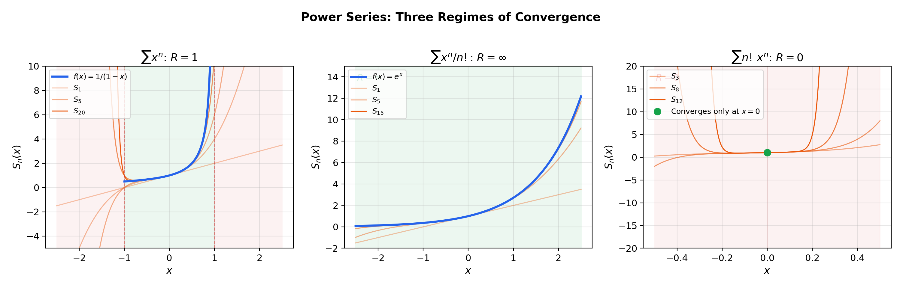
has for all and center . From Series Convergence & Tests, this converges to for and diverges for . This is the prototype: convergence on an open interval, divergence outside it.
📝 Example 2 (The exponential series (R = ∞))
has and converges for all . From Mean Value Theorem & Taylor Expansion, we know this equals . The ratio of consecutive terms is for every fixed , so the ratio test gives convergence everywhere.
📝 Example 3 (A series that converges only at its center (R = 0))
diverges for every . The ratio for any fixed . The “radius of convergence” is — this series is useless as a function of .
💡 Remark 1 (Power series generalize polynomials)
A polynomial of degree is a power series with for . It converges everywhere (). Power series extend this to “infinite-degree polynomials,” but the trade-off is that convergence is no longer automatic.
3. Radius of Convergence
The three examples above illustrate a remarkable structural fact: a power series always converges on an interval centered at . The half-width of this interval is the radius of convergence — and it is determined entirely by the coefficients.
🔷 Theorem 1 (Existence of the Radius of Convergence)
For any power series , exactly one of the following holds:
(i) The series converges only at ().
(ii) The series converges for all ().
(iii) There exists such that the series converges absolutely for and diverges for .
Proof.
Suppose converges at some . Then (by the divergence test from Series Convergence & Tests), so for some bound . For any with , set . Then
Since converges (geometric series with ), the comparison test gives absolute convergence at .
Now define . If the series converges only at , then (case i). If the supremum is infinite, then (case ii). Otherwise, is a positive real number (case iii): the argument above shows convergence for , and divergence for follows because if the series converged at some with , it would also converge at all with , contradicting .
📐 Definition 2 (Radius of Convergence)
The number from Theorem 1 is the radius of convergence of . We allow and . The open interval is the open interval of convergence.
How do we compute ? The root and ratio tests from Series Convergence & Tests, applied to the coefficient sequence, give explicit formulas.
🔷 Theorem 2 (The Cauchy-Hadamard Formula)
with the convention and .
Proof.
Apply the root test from Series Convergence & Tests to :
The root test gives convergence when this is , i.e., , and divergence when , i.e., .
🔷 Theorem 3 (Ratio Test for Radius)
If exists (possibly or ), then
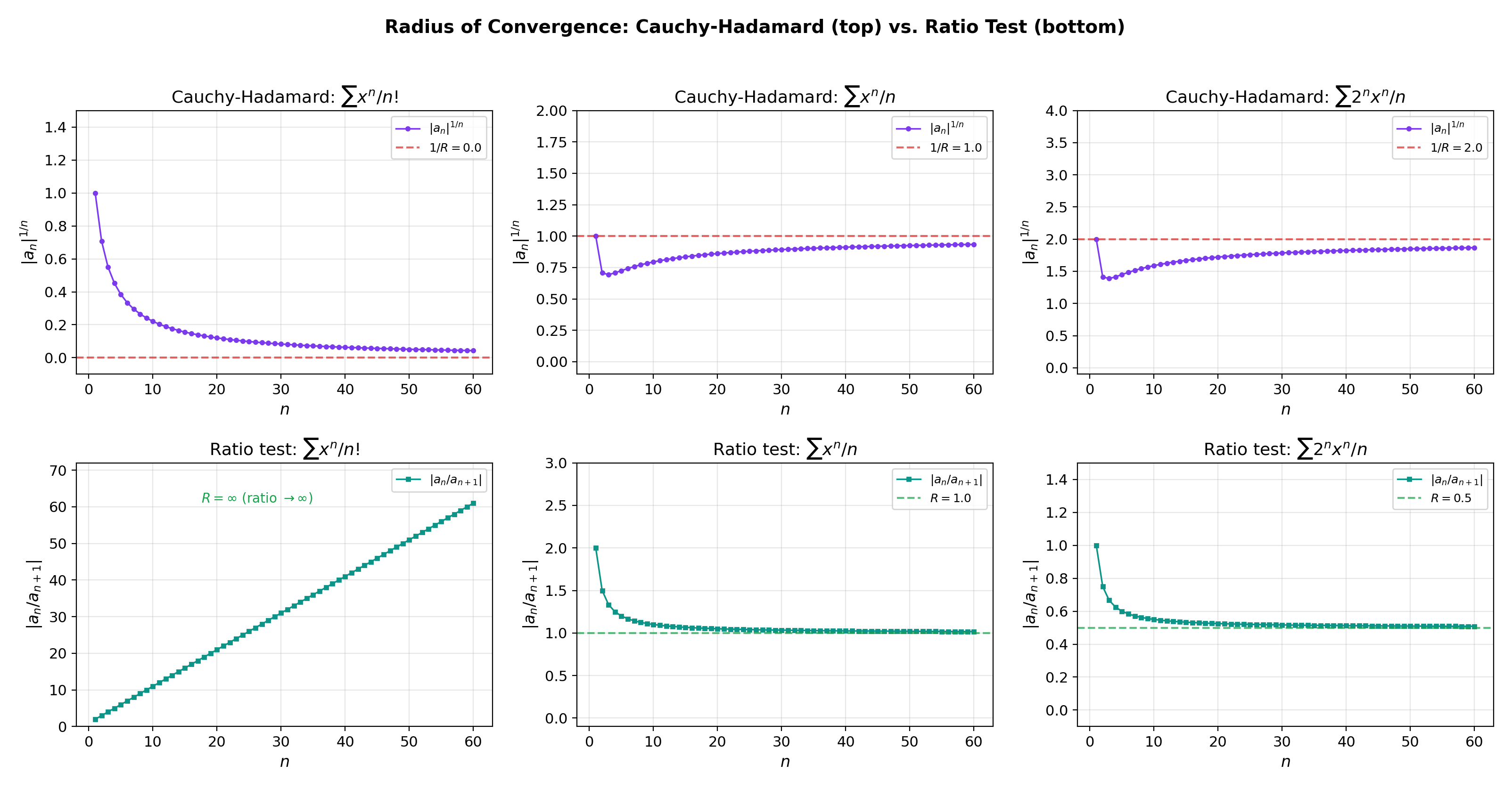
💡 Remark 2 (Root test vs. ratio test)
The Cauchy-Hadamard formula always works (it uses limsup). The ratio test requires the limit to exist. When both apply, they give the same . From Series Convergence & Tests, the root test is strictly stronger — there exist series where the ratio test is inconclusive but the root test determines .
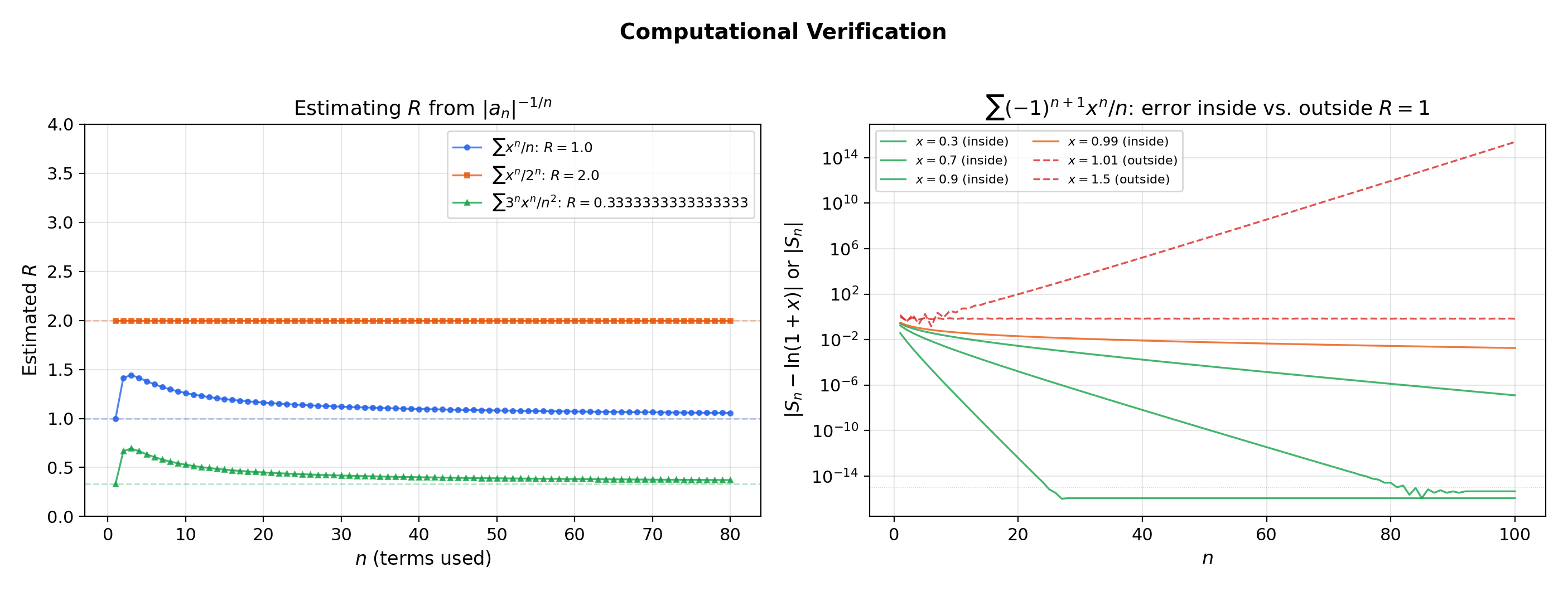
📝 Example 4 (Computing R for standard series)
(a) : ratio gives .
(b) : ratio gives .
(c) : ratio gives .
(d) : ratio gives .
(e) : Cauchy-Hadamard gives , so .
The explorer below lets you see the diagnostic sequences and converging to , and probe what happens when you evaluate the series at points inside and outside the radius.
4. Endpoint Behavior — Where the Tests from Topic 17 Come to Work
The radius determines convergence on the open interval and divergence outside . But at the endpoints themselves, the power series becomes a numerical series — and you must test it directly using the convergence toolkit from Series Convergence & Tests.
📐 Definition 3 (Interval of Convergence)
The interval of convergence of is the set of all where the series converges. It always includes the open interval and may or may not include either endpoint.
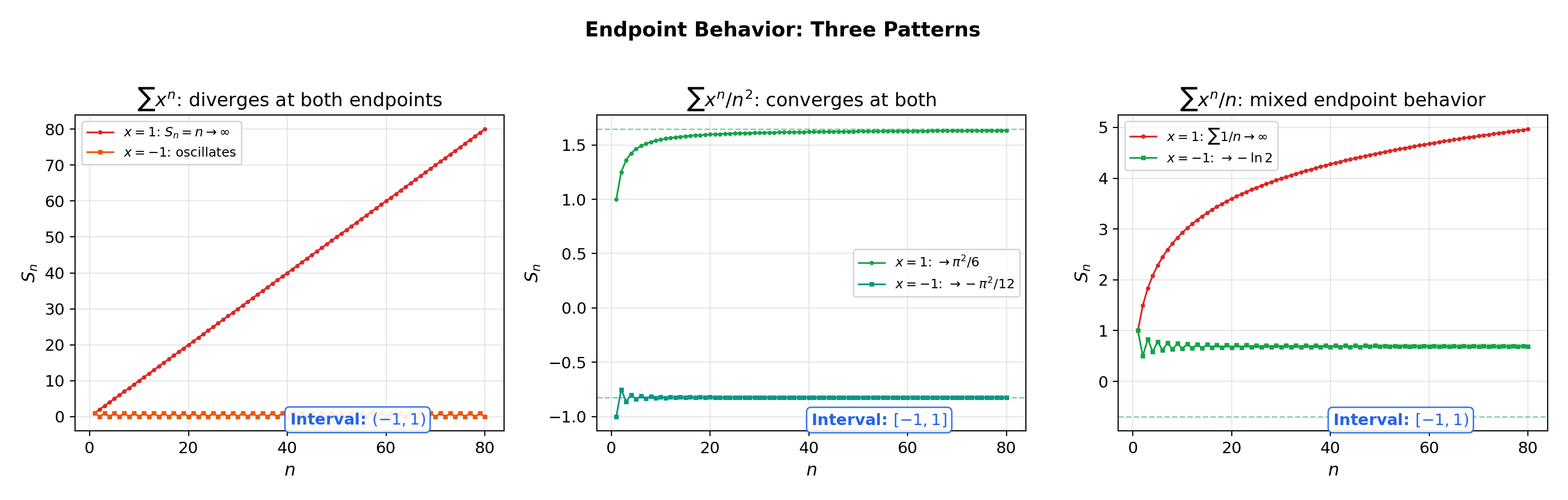
📝 Example 5 (Three endpoint behaviors)
All three of the following have centered at :
(a) : diverges at both endpoints. At : diverges. At : diverges. Interval: .
(b) : converges at both endpoints. At : converges (-series, ). At : converges absolutely. Interval: .
(c) : mixed. At : converges by the alternating series (Leibniz) test. At : diverges (harmonic). Interval: .
💡 Remark 3 (The four endpoint possibilities)
With two endpoints and two possible verdicts (converge/diverge) at each, there are four combinations: , , , . All four occur in practice. The algorithm is always the same: (1) compute via ratio or Cauchy-Hadamard; (2) substitute and apply a convergence test from Series Convergence & Tests.
📝 Example 6 (Endpoint analysis with comparison and alternating series tests)
For , the ratio test gives . At : converges by the Leibniz test (alternating, terms decrease to ). At : diverges by comparison with (-series with ). Interval: .
5. Uniform Convergence on Compact Subsets
This is the section where the threads come together. We connect power series to the uniform convergence theory from Uniform Convergence, establishing the key property that makes everything in the next section work.
🔷 Theorem 4 (Uniform Convergence on Compact Subsets)
If has radius of convergence , then the series converges uniformly on every closed interval for .
Proof.
Fix with and let . For , we have
Since , the series converges (by the definition of — the power series converges absolutely for , and ). By the Weierstrass M-test from Uniform Convergence, the series converges uniformly on .
💡 Remark 4 (Why compact subsets, not the full interval)
The power series converges pointwise on but does not converge uniformly on all of . The partial sums satisfy
for every (the supremum blows up as ). The uniform convergence theorem only guarantees uniformity on for — compact subsets strictly inside the interval of convergence. This is the same pointwise-vs-uniform distinction from Uniform Convergence, now appearing in a concrete power-series context.
![Uniform convergence on compact subsets — sup-norm error decreasing on [-r,r] for r < R](/images/topics/power-taylor-series/uniform-convergence-compact.png)
6. Term-by-Term Differentiation & Integration
Because power series converge uniformly on compact subsets, the interchange theorems from Uniform Convergence apply. We can differentiate and integrate a power series term by term — and the resulting series has the same radius of convergence. This is the computational payoff of the theory.
🔷 Theorem 5 (Term-by-Term Differentiation)
If has radius of convergence , then is differentiable on and
The differentiated series has the same radius of convergence .
Proof.
Fix and choose with . On , the series converges uniformly (Theorem 4). The partial sums are polynomials, hence differentiable. Each .
The differentiated series has
since . So the differentiated series has the same radius and converges uniformly on .
By the interchange theorem for differentiation from Uniform Convergence, .
🔷 Corollary 1 (Power series are C^∞)
Applying Theorem 5 repeatedly, for all , each with radius . A power series is infinitely differentiable inside its radius of convergence.
🔷 Theorem 6 (Term-by-Term Integration)
If has radius , then
for . The integrated series has radius of convergence .
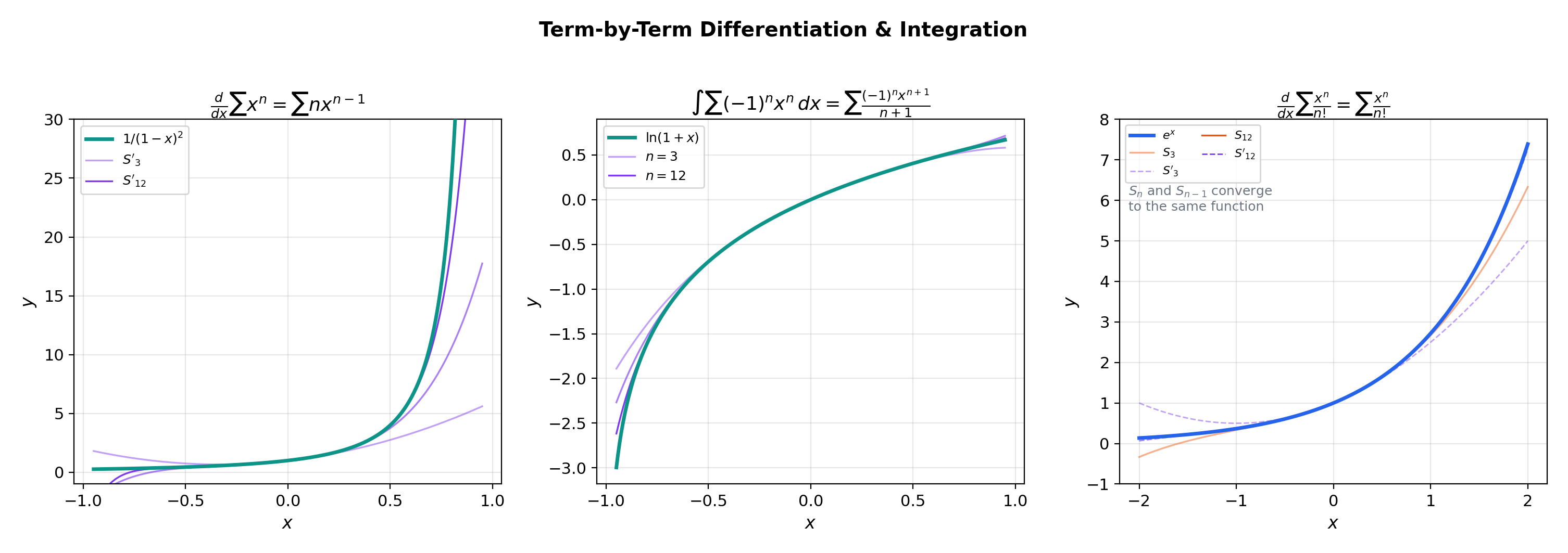
📝 Example 7 (Deriving 1/(1−x)² by differentiation)
Differentiating term by term gives
📝 Example 8 (Deriving ln(1+x) by integration)
Integrate term by term from to :
The series also converges at by the alternating series test (Leibniz) from Series Convergence & Tests, giving .
📝 Example 9 (The arctangent series)
Integrate to get
Setting gives the Leibniz formula .
The explorer below lets you see term-by-term differentiation and integration in action. Toggle between the two modes and watch how the partial sums of the derived/integrated series track the true derivative/integral.
7. Taylor Series as Power Series — The Infinite Extension
A Taylor series is a power series whose coefficients are determined by the derivatives of a function. The question is: when does this particular power series converge to the function?
🔷 Theorem 7 (Coefficient Extraction (Uniqueness))
If on some interval with , then
for all . A power series representation of a function is necessarily its Taylor series.
Proof.
By Corollary 1, . Setting , all terms with vanish (they contain a factor ), leaving . Solving gives .
💡 Remark 5 (Uniqueness has teeth)
If two power series and are equal on any interval containing , then for all . You cannot have two different power series representations of the same function centered at the same point. This makes power series representations canonical.
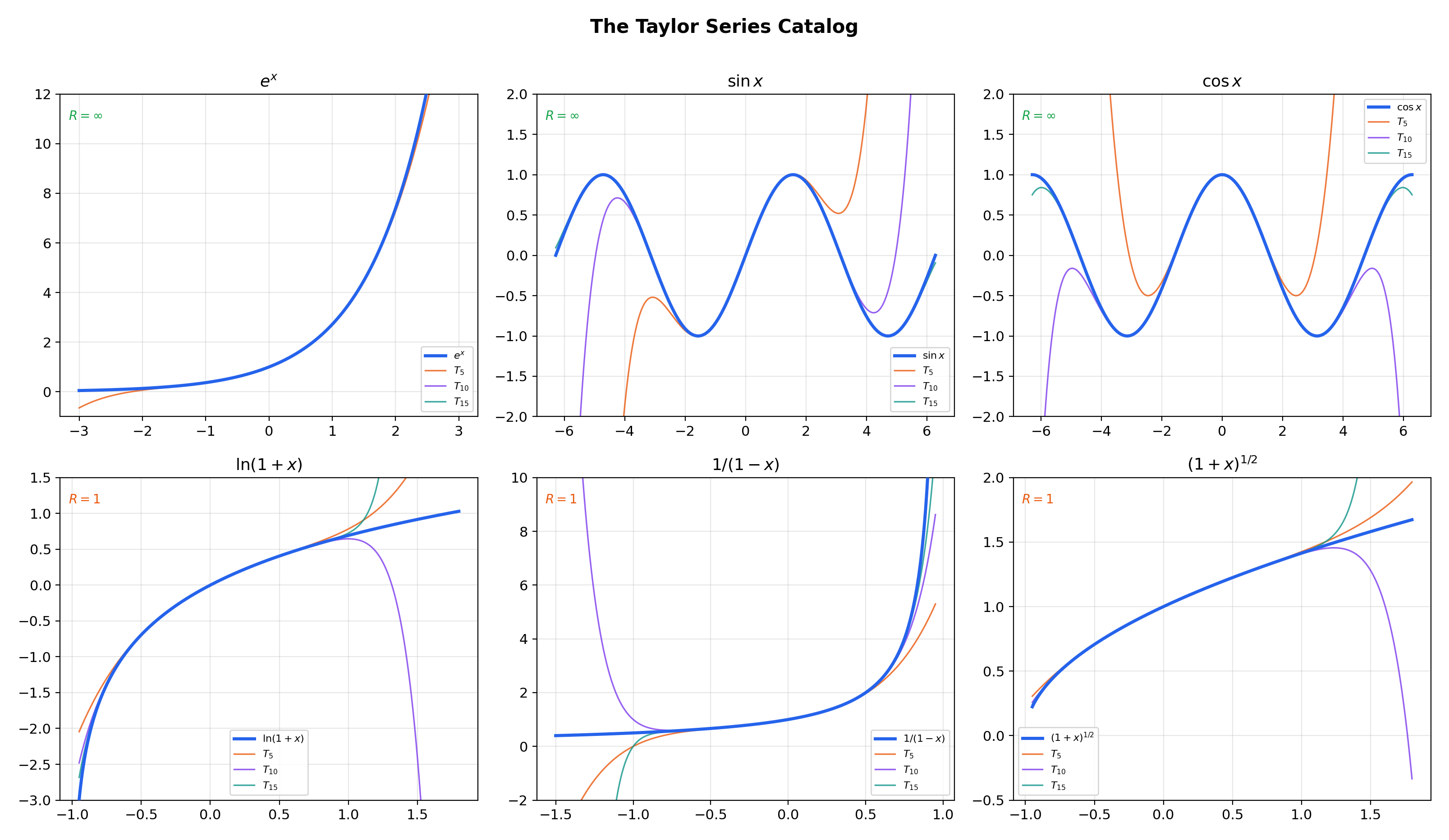
📝 Example 10 (The Taylor series catalog)
The six essential Taylor series at (Maclaurin series):
1. ,
2. ,
3. ,
4. , , also converges at
5. ,
6. (binomial series), for non-integer
The flagship explorer below shows partial sums of these Taylor series converging to their target functions. Select a function, drag the slider, and watch approach inside the radius of convergence — and diverge wildly outside it.
8. Analytic vs. Smooth — When Taylor Series Succeed and Fail
Every power series with defines a function (Corollary 1). But does every function have a convergent Taylor series? The answer is no — and understanding why is the deepest insight of this topic.
📐 Definition 4 (Analytic Function)
A function is real analytic at if its Taylor series at converges to in some neighborhood of :
A function is analytic on an interval if it is analytic at every point of that interval. The class of analytic functions is denoted .
🔷 Theorem 8 (Sufficient Condition for Analyticity)
If is on an interval containing and there exist constants and such that
then is analytic at with .
Proof.
The Lagrange remainder from Mean Value Theorem & Taylor Expansion satisfies
For , this is a geometric sequence converging to , so and the Taylor series converges to .
📝 Example 11 (e^x, sin x, cos x are entire (analytic everywhere))
For : on any interval , . Setting and gives the bound — but we need , and the actual derivatives satisfy the much tighter bound (without the factor). This means for every , so .
The same argument applies to and , where all derivatives are bounded by .
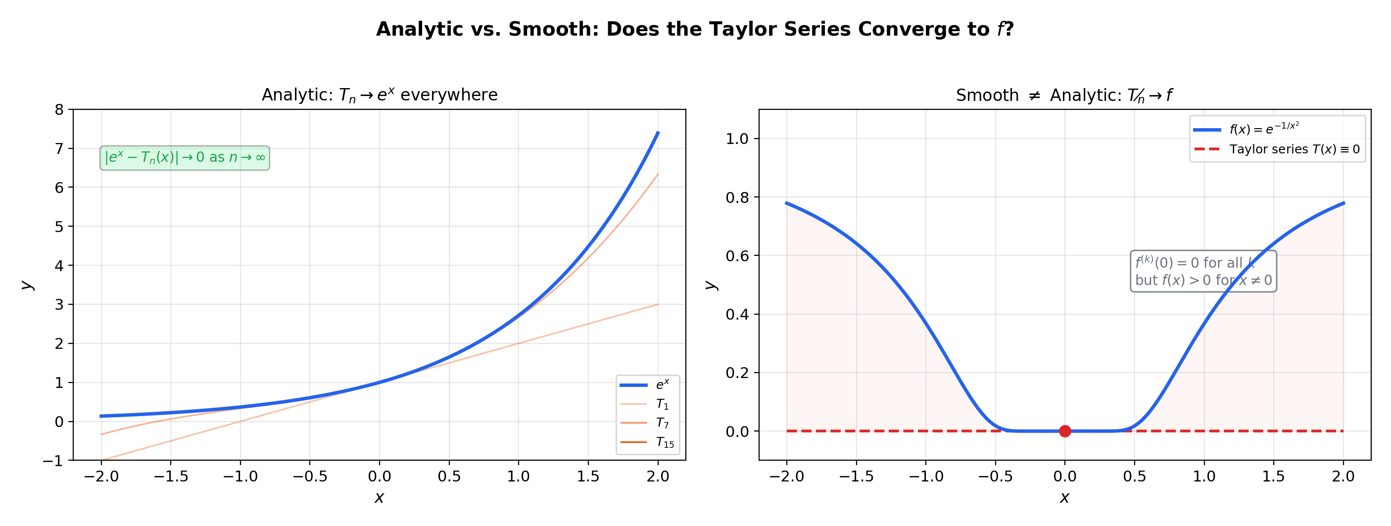
📝 Example 12 (Smooth but not analytic — e^{−1/x²} revisited)
This extends the discussion from Mean Value Theorem & Taylor Expansion, Example 8. Define
All derivatives at are (the proof by induction uses L’Hôpital’s Rule repeatedly: each is a polynomial in times , and decays faster than any polynomial as ). So the Taylor series at is . But for . The Taylor series converges — but to the wrong function.
The derivative bound fails for any finite : the derivatives at points near (but not at ) grow faster than any geometric rate.
💡 Remark 6 (Analytic functions are rare but ubiquitous)
In a precise sense (Baire category), “most” smooth functions are not analytic. Yet in practice — in calculus, physics, and ML — almost every function we encounter is analytic (or piecewise analytic). The standard function zoo (, , , , polynomials, rational functions, compositions thereof) is closed under the operations that preserve analyticity. The smooth-but-not-analytic examples are constructed to violate the derivative growth condition.
9. Connections to Statistics
Taylor series are the asymptotic backbone of statistical theory: characteristic-function CLT proofs, asymptotic normality of the MLE, Laplace approximation, the delta method, and the bias expansions for nonparametric estimators all expand to second order around a critical point and bound the remainder.
Characteristic functions and the CLT
The characteristic-function proof of the CLT expands as a Taylor series in . The dominant terms give the Gaussian characteristic function ; the remainder vanishes as . See formalStatistics Central Limit Theorem.
Delta method and Laplace approximation
The delta method — — is a 1st-order Taylor expansion. Laplace approximation Taylor-expands the log-posterior to 2nd order around the MAP, producing a Gaussian approximation with covariance and the BIC penalty as its asymptotic form. See formalStatistics Expectation & Moments and formalStatistics Bayesian Model Comparison & BMA.
KDE bias and Edgeworth expansions
The KDE bias expansion is a Taylor series in the bandwidth . Bootstrap higher-order accuracy — vs. the CLT’s — follows from matching Edgeworth (Taylor) terms between the bootstrap and true distributions. See formalStatistics Kernel Density Estimation and formalStatistics Bootstrap.
10. Connections to ML — Taylor Expansions in Optimization and Inference
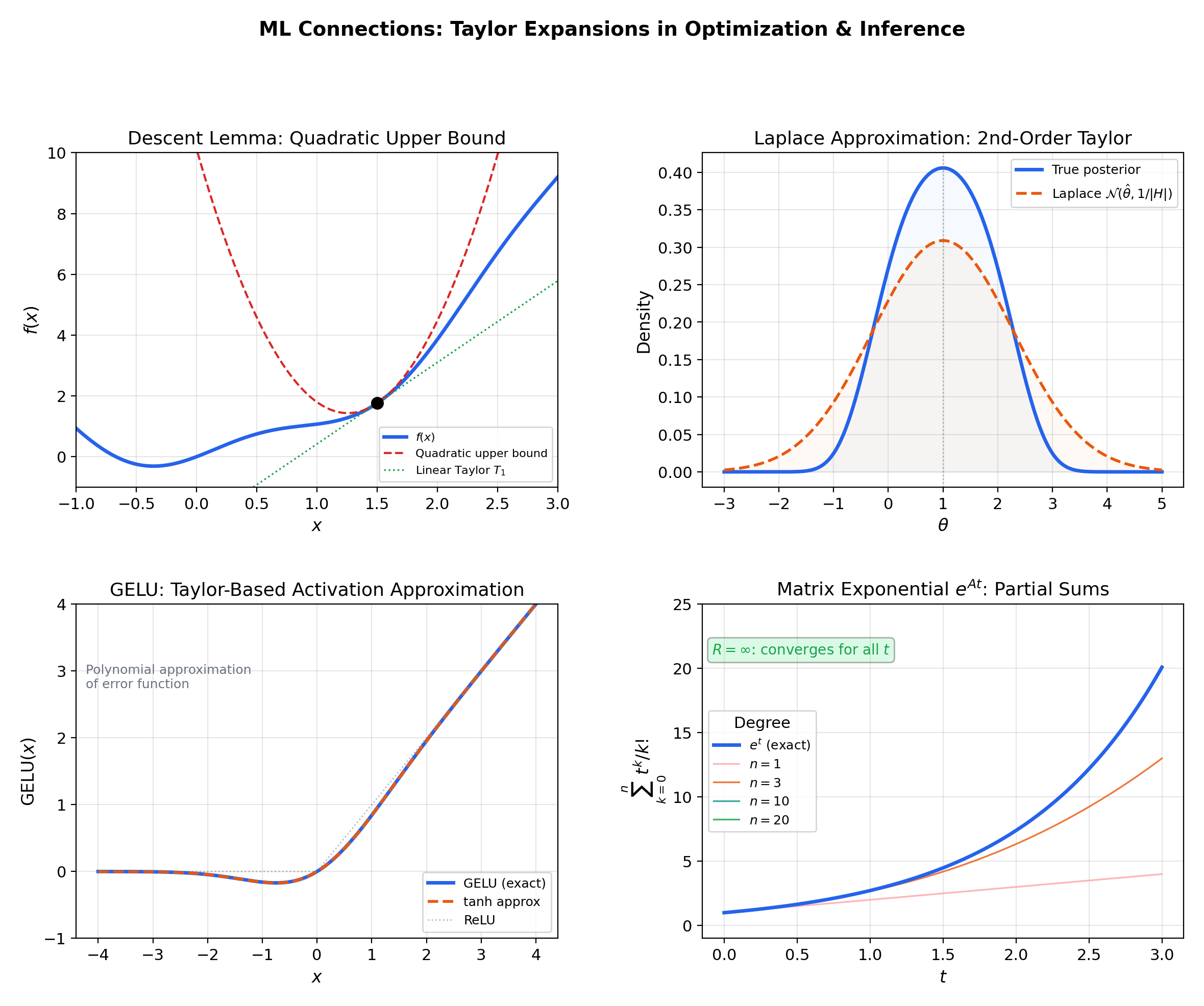
9.1 The descent lemma and gradient descent
If is -Lipschitz continuous, the second-order Taylor expansion with Lagrange remainder gives the descent lemma:
Setting with step size yields
— the fundamental inequality guaranteeing that gradient descent makes progress at every step. Newton’s method goes further: it uses the full quadratic Taylor model as its step direction, achieving quadratic convergence near optima. (→ formalML: Gradient Descent)
9.2 The Laplace approximation
Given a posterior where , the second-order Taylor expansion of at the MAP estimate gives
where . This yields the Gaussian approximation — replacing a complex posterior with a Gaussian centered at the mode. The quality of this approximation depends on how well the second-order Taylor expansion captures the log-posterior, which is exactly the analyticity question this topic addresses. (→ formalML: Information Geometry)
9.3 GELU and activation function approximation
The Gaussian Error Linear Unit , where is the standard normal CDF, is one of the most widely used activation functions in modern transformers. Its practical implementation uses a polynomial approximation:
which is derived from the Taylor expansion of the error function. The coefficient comes from matching Taylor series terms — a direct application of power series truncation in production neural network code.
9.4 Matrix exponential in continuous-time models
For neural ODEs, state-space models (S4, Mamba), and continuous-time dynamical systems, the matrix exponential
is a power series in with matrix coefficients. It converges for all (since for the scalar exponential, and the norm bound gives a convergent comparison series). Term-by-term differentiation gives , which is the fundamental solution to the linear ODE .
11. Computational Notes
- Power series evaluation: Horner’s method. Evaluating naively requires multiplications. Horner’s method rewrites and evaluates from the inside out in with minimal round-off. Use
numpy.polynomial.polynomial.polyvalfor numerical stability. - Radius of convergence estimation. For tabulated coefficients, compute for large and look for convergence to . The tail average of this sequence gives a reliable numerical estimate.
- Endpoint testing is algorithmic. Compute via ratio or Cauchy-Hadamard, then substitute into the series and apply the convergence-test flowchart from Series Convergence & Tests.
Connections & Further Reading
Prerequisites — topics you need first
Uniform Convergence
The Weierstrass M-test (Topic 4) proves that power series converge uniformly on compact subsets of their interval of convergence. The interchange theorems for integration and differentiation (Topic 4) then justify term-by-term calculus — the most powerful computational tool for power series.
Series Convergence & Tests
Power series are series whose terms are functions aₙ(x−c)ⁿ rather than fixed numbers. The ratio test gives R = lim|aₙ/aₙ₊₁|, the root test gives R = 1/limsup|aₙ|^(1/n) (Cauchy-Hadamard), and endpoint analysis uses comparison and alternating series tests — all from Topic 17.
Mean Value Theorem & Taylor Expansion
Topic 6 built Taylor polynomials Tₙ(x) and proved remainder bounds Rₙ(x), but left the question: when does Rₙ(x) → 0 as n → ∞? Topic 18 answers this by characterizing analytic functions — those for which the Taylor series converges to f — and providing the radius-of-convergence framework.
The Riemann Integral & FTC
Term-by-term integration of power series produces antiderivatives expressed as power series. The integral ∫₀ˣ 1/(1+t²)dt = arctan(x) can be computed by integrating the geometric series 1/(1+t²) = ∑(-1)ⁿt²ⁿ term by term, yielding the Leibniz formula arctan(x) = ∑(-1)ⁿx^(2n+1)/(2n+1).
Improper Integrals & Special Functions
Power series with infinite radius of convergence (eˣ, sin x, cos x) define entire functions whose improper integrals are computed via term-by-term integration. The Gaussian integral ∫e^(−x²)dx is evaluated by expanding e^(−x²) as a power series and integrating term by term.
Where this leads — next in formalCalculus
Fourier Series & Orthogonal Expansions
Trigonometric series as a generalization of power series using sin and cos instead of monomials — the two approximation paradigms (local analytic vs. global periodic) are unified in approximation theory.
Approximation Theory
Weierstrass approximation theorem and non-Taylor polynomial approximations — the theoretical ceiling that Taylor expansion reaches toward but doesn't always hit.
Linear Systems & Matrix Exponential
The matrix exponential e^(At) = Σ (At)^k/k! is a power series solution to ẋ = Ax — everything about convergence and term-by-term manipulation here carries over directly.
On to formalStatistics — where this calculus powers inference
Central Limit Theorem
The characteristic-function proof of the CLT expands log φ_{X_i}(t/√n) as a Taylor series in t. The dominant terms give the Gaussian characteristic function e^(-σ²t²/2); the remainder terms vanish as n → ∞.
Expectation Moments
The delta method: if √n(θ̂ - θ) ⟹ N(0, σ²) and g is differentiable, then √n(g(θ̂) - g(θ)) ⟹ N(0, [g'(θ)]² σ²). The proof is a 1st-order Taylor expansion g(θ̂) = g(θ) + g'(θ)(θ̂ - θ) + o_p(1/√n).
Bayesian Model Comparison And Bma
Laplace approximation Taylor-expands the log-posterior to second order around the MAP. The resulting Gaussian approximation has covariance matrix (-∇²ℓ)⁻¹. BIC's asymptotic derivation rests on the higher-order error term of this expansion.
Kernel Density Estimation
The KDE bias expansion E[f̂_n(x)] - f(x) = (h²/2) f''(x) μ_2(K) + O(h⁴) is a Taylor series in the bandwidth h. The dominant bias term gives the asymptotic MSE; the optimal bandwidth h* balances bias² against variance.
Bootstrap
The Edgeworth expansion of √n(θ̂_n - θ) uses Taylor series in the characteristic function. Bootstrap higher-order accuracy — O(n⁻¹) vs. the CLT's O(n^(-1/2)) — follows from matching Edgeworth terms between the bootstrap and true distributions.
Order Statistics And Quantiles
The Bahadur representation of sample quantiles, ξ̂_p = ξ_p - (F_n(ξ_p) - p)/f(ξ_p) + o_p(n^{-1/2}), is a Taylor-series-flavored asymptotic — a first-order linearization of the inverse-CDF map around the true quantile.
Continuous Distributions
The Normal MGF derivation uses 'completing the square' in the exponent, and the Gamma function's properties connect to power-series representations. The exponential series $e^x = \sum x^k/k!$ underwrites the MGF identity $M_X(t) = \sum \mathbb E[X^k]\,t^k/k!$ for distributions with finite moments.
Discrete Distributions
The exponential power series $e^x = \sum x^k/k!$ verifies that the Poisson PMF sums to 1 and drives MGF derivations. The probability generating function $G_X(s) = \mathbb E[s^X] = \sum p_k s^k$ is a power series whose coefficients are the PMF values.
Exponential Families
The log-partition function's moment-generating properties use Taylor-expansion arguments. The relationship between $A(\eta)$ and the moment-generating function connects to power series — $A'(\eta) = \mathbb E[T(X)]$ and $A''(\eta) = \mathrm{Var}(T(X))$ are the first two Taylor coefficients of $A$ at $\eta$.
Generalized Linear Models
GLM asymptotic-normality (§22.3 Thm 3) and the deviance LRT $\to \chi^2_k$ (§22.7 Thm 6) both rest on multivariate Taylor expansions of the log-likelihood around the MLE. The $\sqrt n$ scaling in the asymptotic distribution is exactly the Taylor-series remainder bound.
On to formalML — where this calculus powers ML
Gradient Descent
The descent lemma f(y) ≤ f(x) + ∇f(x)ᵀ(y−x) + L/2·‖y−x‖² is a second-order Taylor expansion with L-Lipschitz gradient remainder bound. Newton's method replaces gradient descent's linear Taylor model with the full quadratic Taylor model T₂(x), achieving quadratic convergence near optima.
Convex Analysis
A twice-differentiable function is convex iff its first-order Taylor expansion is a global lower bound: f(y) ≥ f(x) + ∇f(x)ᵀ(y−x). This characterization follows directly from Taylor's theorem with non-negative second derivative.
Information Geometry
The Fisher information matrix I(θ) is the Hessian of the KL divergence at θ = θ₀, computed via second-order Taylor expansion. The resulting Riemannian metric on parameter space is the foundation of natural gradient methods.
Smooth Manifolds
The smooth-vs-analytic distinction developed here is foundational: analytic functions are locally representable by convergent power series in coordinate charts, while smooth functions form the more general C^∞ category used in differential geometry.
References
- book Rudin (1976). Principles of Mathematical Analysis Chapter 8 — the definitive treatment of power series, uniform convergence on compact subsets, and the algebra of power series
- book Abbott (2015). Understanding Analysis Chapter 6 — power series and Taylor series with an emphasis on the role of uniform convergence in justifying interchange
- book Spivak (2008). Calculus Chapter 23 — Taylor series with complete proofs of term-by-term theorems and the analytic vs. smooth distinction
- book Folland (1999). Real Analysis: Modern Techniques and Their Applications Section 0.6 — power series in the context of analysis prerequisites for measure theory
- book Bartle & Sherbert (2011). Introduction to Real Analysis Chapter 9 — power series convergence with careful attention to endpoint behavior and applications
- paper Hendrycks & Gimpel (2016). “Gaussian Error Linear Units (GELUs)” GELU(x) = x·Φ(x) is approximated via its Taylor expansion 0.5x(1 + tanh(√(2/π)(x + 0.044715x³))) — a direct application of power series truncation in neural network activation design.
- paper MacKay (1992). “A Practical Bayesian Framework for Backpropagation Networks” The Laplace approximation replaces the posterior with a Gaussian centered at the MAP estimate using a second-order Taylor expansion of the log-posterior — a foundational Bayesian ML technique.