Sequences, Limits & Convergence
The rigorous foundation of calculus — making 'arbitrarily close' precise with the ε-N definition, and the convergence theorems that guarantee your algorithms actually converge
Abstract. A sequence in ℝ is a function a: ℕ → ℝ. We say (aₙ) converges to L if for every ε > 0, there exists N ∈ ℕ such that n ≥ N implies |aₙ - L| < ε. This definition — the ε-N definition — is where calculus becomes rigorous. The Monotone Convergence Theorem guarantees that every bounded monotone sequence converges, the Squeeze Theorem lets us establish limits by trapping a sequence between two convergent bounds, and the Algebra of Limits lets us decompose complex limits into simpler pieces. The Bolzano-Weierstrass Theorem — every bounded sequence has a convergent subsequence — is the compactness result that underpins the existence of minimizers in optimization. Cauchy sequences provide a criterion for convergence that does not require knowing the limit in advance, and the completeness of ℝ (every Cauchy sequence converges) is the structural property that makes calculus work. For machine learning, gradient descent θₜ₊₁ = θₜ - η∇f(θₜ) defines a sequence whose convergence is the entire point; the rate of convergence — sublinear O(1/n) for SGD, linear O(rⁿ) for GD on strongly convex functions, quadratic for Newton's method — determines practical algorithm selection. The Robbins-Monro conditions on learning rate schedules (Σηₜ = ∞, Σηₜ² < ∞) are statements about series convergence that we formalize here.
Overview & Motivation
You’ve watched a training loss curve drop toward zero and level off. You’ve seen gradient descent “converge.” You’ve tuned a learning rate schedule until the optimizer “settles down.” But what do any of these phrases actually mean?
When we say a sequence of iterates converges, we’re making a precise mathematical claim: no matter how tight a tolerance you specify — a billionth, a trillionth, any positive number at all — there is some point in the sequence past which every single term stays within that tolerance of the limit. This is the - definition, and it is where calculus becomes rigorous.
In this topic, we build the complete machinery of sequence convergence from scratch. We start with what a sequence is, move to the - definition that makes “arbitrarily close” precise, prove the core convergence theorems that let us establish limits without computing them directly, and develop the Cauchy criterion that lets us detect convergence without even knowing the limit. Every theorem here has a direct application to machine learning — gradient descent convergence, optimizer guarantees, and the learning rate conditions that make stochastic methods work.
Sequences in ℝ
We begin with the most basic object in analysis: a sequence.
📐 Definition 1 (Sequence)
A sequence in is a function . We write or simply for the sequence, where denotes the -th term.
The notation is important: with parentheses denotes the entire sequence as an object, while without parentheses denotes a single term. We’ll be careful about this distinction throughout.
Here are four sequences that appear constantly in machine learning:
- — the simplest decaying sequence. Learning rate schedules like produce sublinear convergence rates for SGD.
- — converges to Euler’s number . The natural exponential shows up in softmax, cross-entropy loss, and the exponential family of distributions.
- — geometric (exponential) decay. This is the momentum coefficient in Adam (), the discount factor in reinforcement learning, and the convergence rate of gradient descent on strongly convex functions.
- — oscillates but converges to . SGD with noisy gradients exhibits exactly this kind of oscillating convergence.
Learning rate schedule: η_t = c/t gives O(1/√t) SGD convergence
📐 Definition 2 (Bounded Sequence)
A sequence is bounded if there exists such that for all . Equivalently, the range is a bounded subset of .
📐 Definition 3 (Monotone Sequence)
A sequence is increasing (or non-decreasing) if for all . It is decreasing (or non-increasing) if for all . A sequence that is either increasing or decreasing is called monotone.
Among our examples: is decreasing, is increasing (a non-trivial fact we’ll use later), is decreasing, and is neither increasing nor decreasing — it oscillates. Monotonicity is a powerful structural property: as we’ll prove shortly, any bounded monotone sequence must converge.
The ε-N Definition of Convergence
We now make the informal idea of “getting arbitrarily close” fully rigorous. This is the definition that separates calculus from hand-waving.
Building the intuition
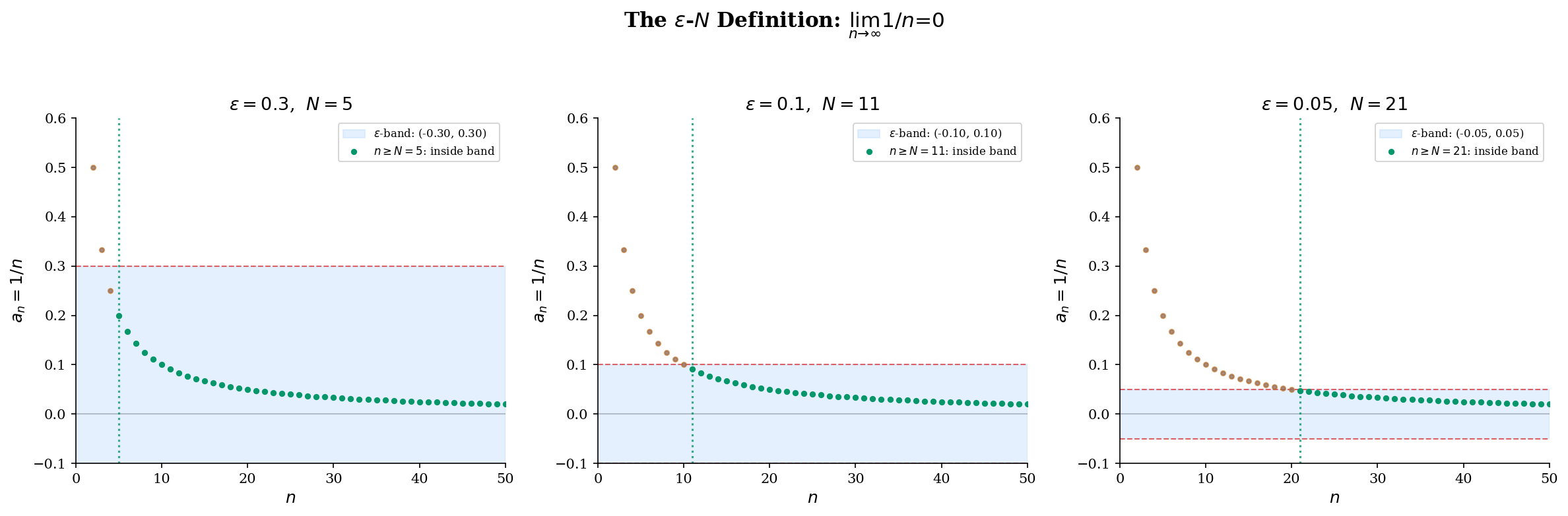
Consider the sequence . Intuitively, the terms are “approaching .” But what does “approaching” mean precisely?
Here’s the key idea: pick any tolerance — say . Then past , every term satisfies . Pick a tighter tolerance, . Then past , every term satisfies . No matter how small a positive you choose, there is always some index past which all terms lie within of .
The formal definition
📐 Definition 4 (Convergence of a Sequence)
A sequence converges to if for every , there exists such that
We write , or , or as .
A sequence that does not converge is called divergent.
Read it carefully: the quantifier structure is . The order matters: is chosen first (by an adversary, if you like), and then we must produce an that works for that . Different values of may require different values of — and smaller generally requires larger .
A complete proof from the definition
📝 Example 1 (Proof that lim 1/n = 0)
Claim: .
Proof. Let be given. We need to find such that implies .
Since , the condition is equivalent to . By the Archimedean property of , there exists with .
Then for all :
Since was arbitrary, we have .
Notice the structure: let be given, choose in terms of , verify the bound. Every - proof follows this template. The creative part is choosing — often this requires algebraic manipulation of the target inequality to isolate .
Two fundamental properties of convergent sequences
🔷 Proposition 1 (Uniqueness of Limits)
If converges, the limit is unique. That is, if and , then .
Proof.
Suppose and . Let be given. Since , there exists such that implies . Since , there exists such that implies .
Let . For any , by the triangle inequality:
Since for every , and is a fixed non-negative number, we must have , i.e., .
This proof uses a technique you’ll see throughout analysis: to show a non-negative quantity equals zero, show it’s less than every positive number. The triangle inequality is the workhorse — it lets us split a distance into two pieces we can control separately.
🔷 Proposition 2 (Convergent Implies Bounded)
Every convergent sequence is bounded.
Proof.
Suppose . Apply the definition with : there exists such that implies , which gives for all .
Set . Then for all .
The converse is false — the sequence is bounded (by ) but not convergent. Boundedness is necessary for convergence, but not sufficient. We need additional structure (like monotonicity) to guarantee convergence.
Convergence Theorems
With the definition established, we now prove three theorems that are the main tools for establishing that a sequence converges. In practice, very few limits are proved directly from the - definition — instead, we use these theorems.
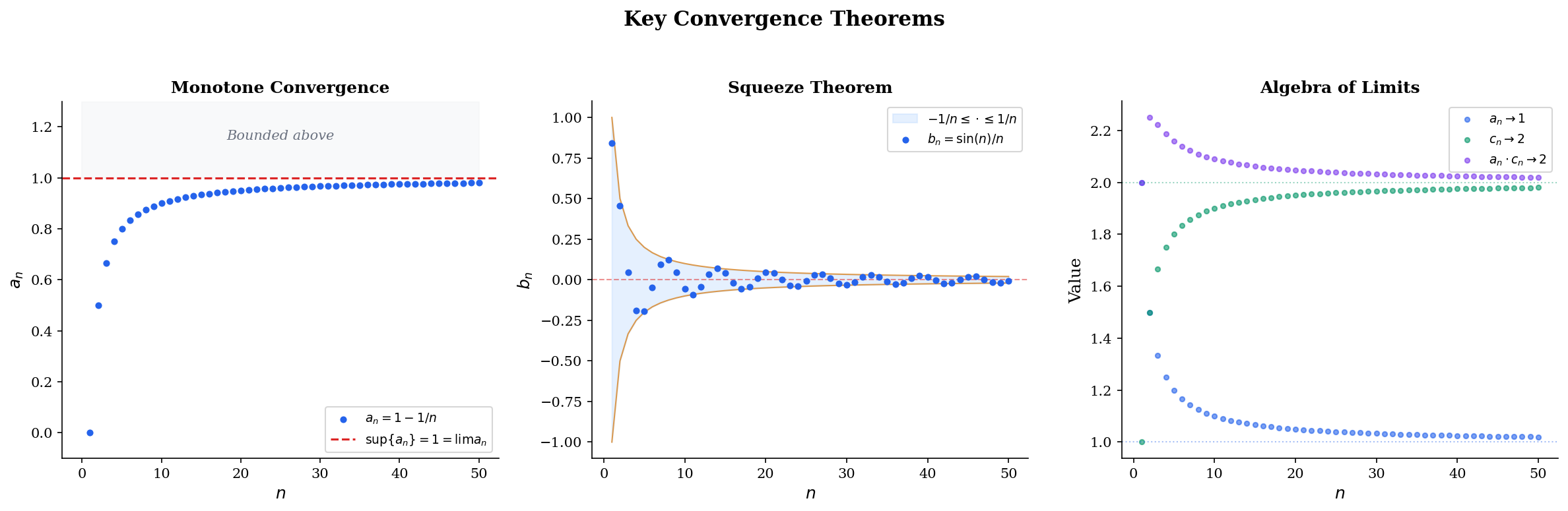
🔷 Theorem 1 (Monotone Convergence Theorem)
Every bounded, monotone sequence in converges.
More precisely: if is increasing and bounded above, then . If is decreasing and bounded below, then .
Proof.
We prove the increasing case; the decreasing case follows by considering .
Let be increasing and bounded above. The set is non-empty and bounded above, so by the completeness axiom (least upper bound property of ), exists.
We claim . Let . Since is the least upper bound of , the number is not an upper bound. Therefore, there exists such that .
Since is increasing, for all :
The first inequality uses our choice of , the second uses with monotonicity, the third uses . Together: for all .
This proof reveals something deep: the Monotone Convergence Theorem is really a theorem about the completeness of . In the rational numbers , the sequence (decimal approximations to ) is increasing and bounded above, but it does not converge in — the limit is irrational. The real numbers were constructed to fill these gaps.
Why this matters for ML: Most gradient descent convergence proofs follow this pattern. If you can show that the loss sequence is decreasing (which requires a sufficiently small step size) and bounded below (e.g., ), the Monotone Convergence Theorem guarantees that the loss converges to some value. Whether that value is the global minimum is a separate question.
🔷 Theorem 2 (Squeeze Theorem)
Let , , and be sequences satisfying for all (or for all past some index). If , then .
Proof.
Let . Since , there exists such that implies , i.e., . Since , there exists such that implies , i.e., .
Let . For :
so .
The Squeeze Theorem is how we prove convergence rates: if we can trap the error between zero and a sequence that decays at a known rate, the Squeeze Theorem tells us decays at least that fast.
🔷 Theorem 3 (Algebra of Limits)
If and , then:
- , provided
- for any constant
Proof.
We prove part (2), the product rule, which is the most instructive case.
Since , the sequence is bounded (Proposition 2): there exists with for all .
Let . Choose such that implies . Choose such that implies .
For :
The key trick: we added and subtracted to create two pieces — one controlled by (using the bound on ) and one controlled by (using the known value of ).
💡 Remark 1
These three theorems are exactly the tools that gradient descent convergence proofs use. Monotone Convergence handles the “loss is decreasing and bounded below” argument. Squeeze establishes convergence rates by bounding the error between known decay rates. Algebra of Limits lets us decompose complex update rules into simpler pieces whose limits we already know.
Subsequences & Bolzano-Weierstrass
Sometimes a sequence doesn’t converge, but parts of it do. This observation leads to one of the most important theorems in analysis.
📐 Definition 5 (Subsequence)
A subsequence of is a sequence where is a strictly increasing sequence of natural numbers.
For example, the even-indexed terms form a subsequence. So do the terms at prime indices . The key constraint is that the indices must be strictly increasing — we must move forward through the original sequence.
🔷 Proposition 3 (Subsequences Inherit Limits)
If , then every subsequence .
Proof.
Let . Since , there exists such that implies .
Since is strictly increasing with , a simple induction shows for all . Therefore, for , we have , so .
The contrapositive gives a powerful divergence test: if two subsequences converge to different limits, the original sequence diverges. For , the even terms and the odd terms . Since the subsequential limits disagree, diverges.
🔷 Theorem 4 (Bolzano-Weierstrass Theorem)
Every bounded sequence in has a convergent subsequence.
Proof.
Let be bounded, so for some interval . We construct a convergent subsequence by repeated bisection.
Step 1. Bisect into and where . At least one half contains infinitely many terms of (if both halves contained only finitely many, the total would be finite, contradicting the fact that the sequence has infinitely many terms). Choose the half containing infinitely many terms. Pick such that .
Step 2. Bisect into two halves. Again, at least one half contains infinitely many terms of . Choose that half and pick such that .
Continuing inductively: At step , we have an interval of length containing infinitely many terms, and an index with .
Convergence. The nested intervals satisfy (increasing left endpoints) and (decreasing right endpoints), and . By the Monotone Convergence Theorem, both and converge, and they must converge to the same limit (since their difference tends to ).
Since for all , the Squeeze Theorem gives .
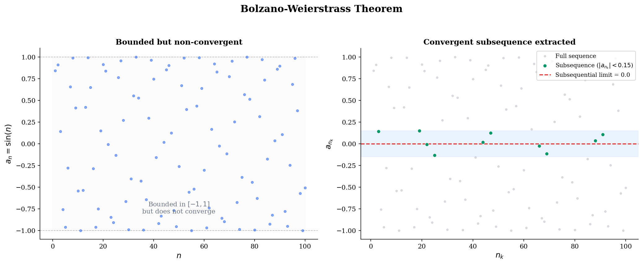
💡 Remark 2
Bolzano-Weierstrass is the one-dimensional version of the compactness argument that guarantees the existence of minimizers in optimization. Here’s the connection: if is continuous and is closed and bounded (compact), then attains its minimum on . The proof works by taking a sequence in with , extracting a convergent subsequence by Bolzano-Weierstrass (generalized to ), and using continuity to show the subsequential limit is a minimizer.
In machine learning, this is why we often restrict the parameter space (weight decay, norm constraints, compact domains) — compactness guarantees that minimizers exist.
Cauchy Sequences & Completeness
The - definition requires us to know the limit in advance. But in practice, we often want to prove convergence without knowing the limit — for instance, we want to show that gradient descent converges to some critical point without identifying which one. The Cauchy criterion solves this problem.
📐 Definition 6 (Cauchy Sequence)
A sequence is a Cauchy sequence if for every , there exists such that
In words: the terms of the sequence get arbitrarily close to each other, not just to some external limit.
Compare with the convergence definition: convergence says terms get close to ; Cauchy says terms get close to each other. The Cauchy condition is intrinsic — it refers only to the sequence itself.
🔷 Proposition 4 (Convergent Implies Cauchy)
Every convergent sequence is Cauchy.
Proof.
Suppose . Let . There exists such that implies . For :
The deep question is the converse: is every Cauchy sequence convergent? In , the answer is no — the decimal approximations to form a Cauchy sequence in that does not converge in . But in , the answer is yes, and this is the whole point of the real number system.
🔷 Theorem 5 (Completeness of ℝ)
Every Cauchy sequence in converges. Equivalently, is a complete metric space.
Proof.
Let be Cauchy in .
Step 1: is bounded. Apply the Cauchy condition with : there exists such that implies . In particular, for all . Setting , we get for all .
Step 2: Extract a convergent subsequence. Since is bounded, Bolzano-Weierstrass gives a subsequence with for some .
Step 3: The full sequence converges to . Let . Since is Cauchy, there exists such that implies . Since , there exists such that implies .
Choose with (possible since ). For any :
The first term is controlled by the Cauchy condition (both and are ), and the second by the subsequential convergence.
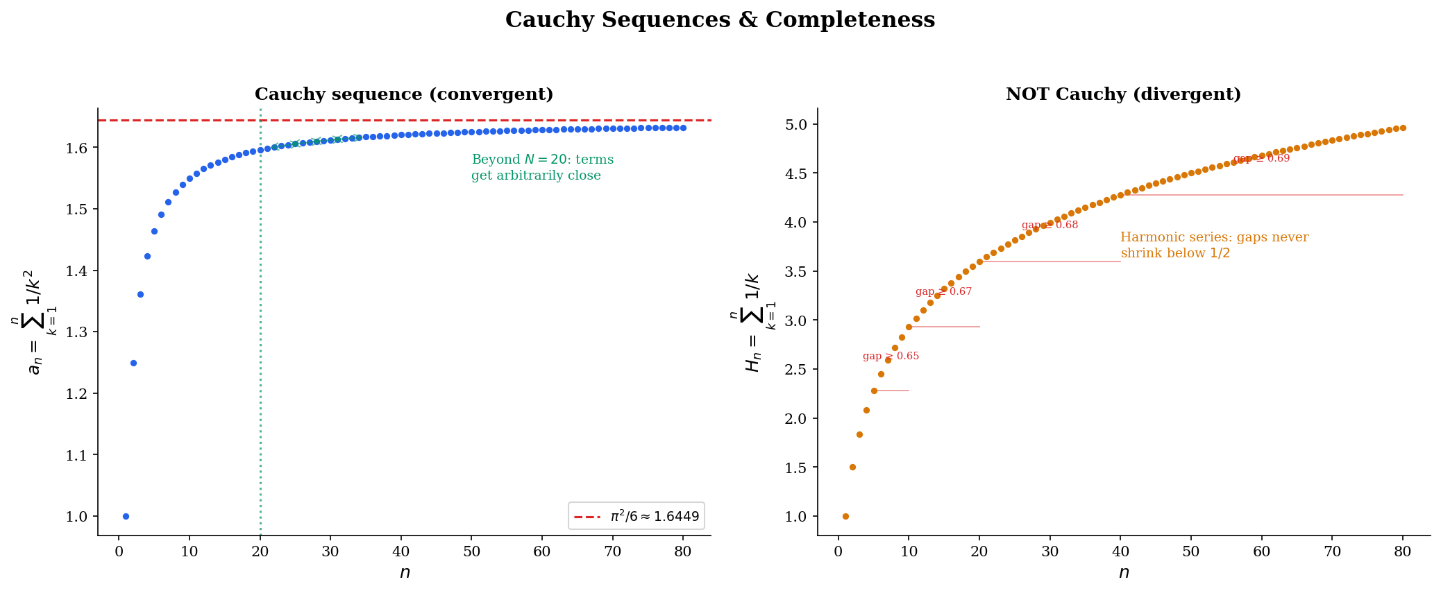
max |am − an| for m,n ≥ 20: 0.0320
max |am − an| for m,n ≥ 20: 1.0655
💡 Remark 3
The Cauchy criterion is the tool of choice when you don’t know the limit. In optimization, we often prove convergence by showing that successive iterates satisfy — this is close to (though not identical to) the Cauchy condition. The completeness of (or ) then guarantees that the iterates converge to some point, even though we may not have a closed-form expression for it.
This is also why completeness matters for function spaces in machine learning. When we optimize over a function class , the class needs to be complete (or at least have compact sublevel sets) to guarantee that minimizing sequences converge to actual minimizers within , not to some function outside it.
Rates of Convergence
Knowing that a sequence converges is important, but often not enough. In practice, we need to know how fast it converges — the difference between and convergence is the difference between an algorithm that takes hours and one that takes seconds.
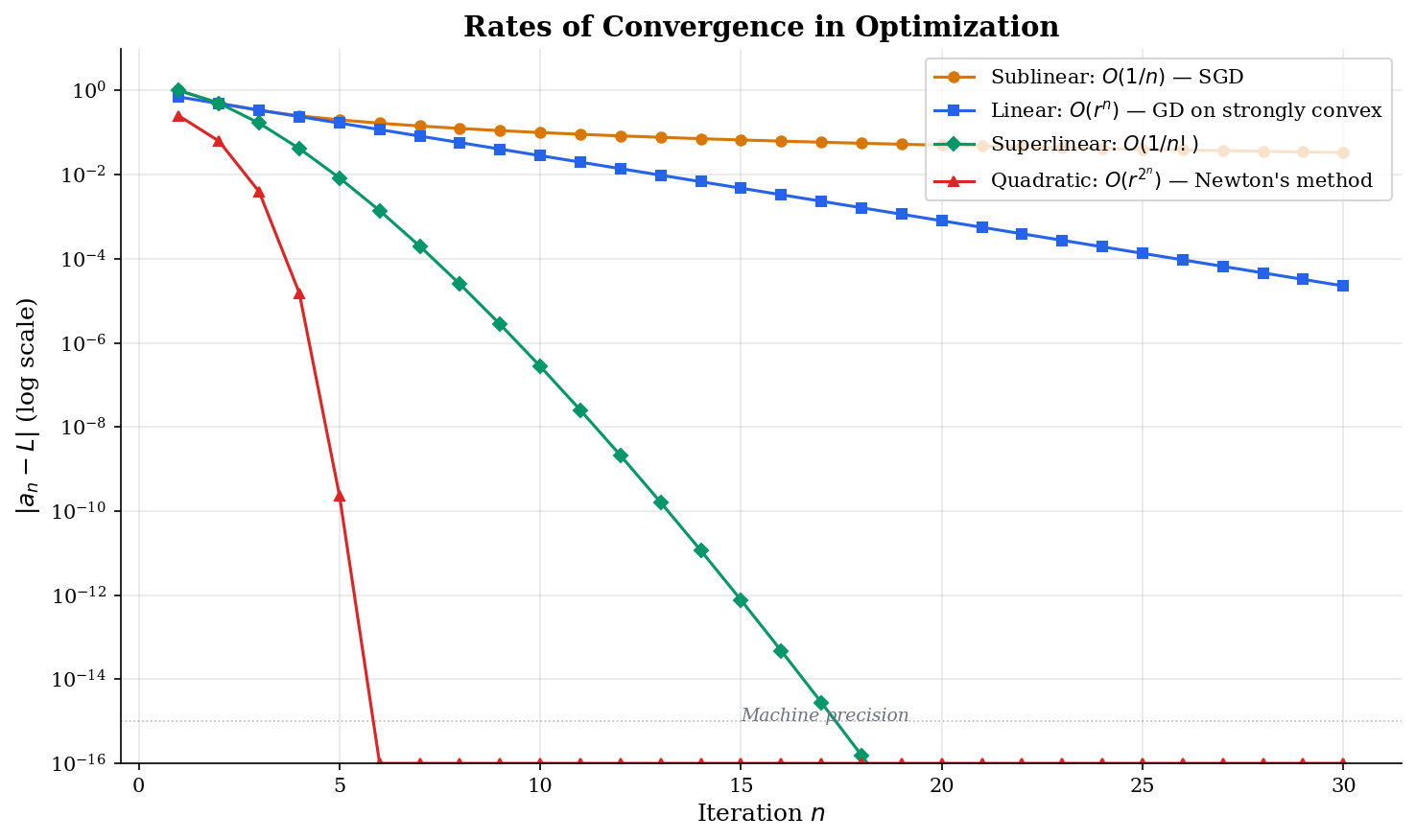
📐 Definition 7 (Rates of Convergence)
Let with errors . The rate of convergence is classified as:
- Sublinear: for some (errors decay polynomially).
- Linear: for some (errors decay by a constant factor each step).
- Superlinear: (the ratio of successive errors tends to zero).
- Quadratic: for some (errors are squared each step — extremely fast).
These rates form a strict hierarchy: quadratic superlinear linear sublinear (in terms of speed). The practical implications are dramatic:
📝 Example 2 (SGD on Convex Functions — Sublinear Rate)
Stochastic gradient descent on a convex function with step size achieves . This is sublinear: halving the error requires quadrupling the number of iterations. For SGD to reach -accuracy, we need steps.
📝 Example 3 (GD on Strongly Convex Functions — Linear Rate)
Gradient descent on a -strongly convex, -smooth function with step size achieves where . This is linear (also called “geometric” or “exponential”) convergence: each step reduces the error by the constant factor . The condition number determines how fast — , so well-conditioned problems ( small) converge faster.
📝 Example 4 (Newton's Method — Quadratic Rate)
Newton’s method for solving near a root achieves once the iterates are sufficiently close to . This is quadratic: if , then , and . The number of correct digits doubles each step.
Connections to Statistics
This topic is the most heavily-cited prerequisite across all of formalStatistics: every limit theorem and every consistency result is a sequence-limit statement at heart.
Convergence of estimators
The (weak and strong) Law of Large Numbers is a sequence-limit theorem for random variables. Consistency of the MLE — — is a sequence-limit statement using the same Cauchy-criterion and monotone-convergence arguments developed here. See formalStatistics Law of Large Numbers and formalStatistics Maximum Likelihood.
Convergence in distribution
The CLT is a convergence-in-distribution statement: the CDFs converge pointwise to at every continuity point. The ε-N framework here is what makes “converges in distribution” precise. The same machinery underwrites every mode of probabilistic convergence: in probability, almost surely, in , in distribution. See formalStatistics Modes of Convergence and formalStatistics Central Limit Theorem.
Bootstrap and empirical processes
Bootstrap consistency asserts that the bootstrap distribution of converges in distribution to the limit of — a sequence limit of empirical measures. Donsker’s theorem extends this to function-valued sequences (the empirical process ). See formalStatistics Bootstrap and formalStatistics Empirical Processes.
Connections to ML
Everything we’ve developed — the - definition, the convergence theorems, the Cauchy criterion, convergence rates — is the mathematical engine behind optimization and learning theory in machine learning.
Gradient descent as a convergent sequence
Consider minimizing . Gradient descent with step size produces the update . This is a geometric sequence:
For , we have , so by the geometric series argument — the errors decay linearly with rate . For or , the sequence diverges. Try it below:
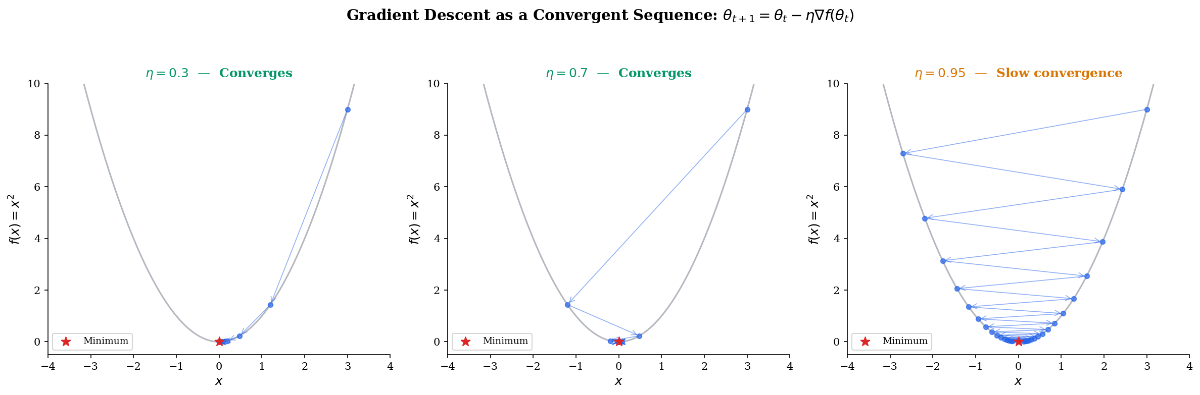
This is why the learning rate matters: too small and convergence is glacially slow ( close to ), too large and the sequence diverges, and there’s an optimal that minimizes . For , the optimal is , giving — convergence in one step.
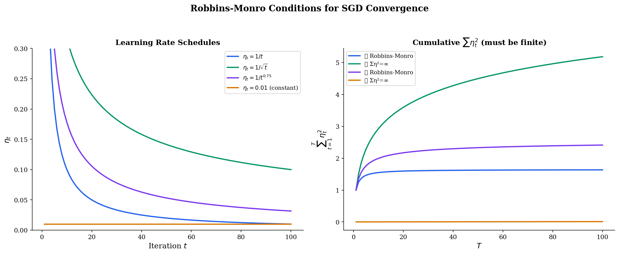
Learning rate schedules & Robbins-Monro
For stochastic gradient descent, a fixed learning rate doesn’t work — the noise prevents convergence to a point. Instead, we need a decaying schedule satisfying the Robbins-Monro conditions:
The first condition () ensures the steps are large enough to reach the optimum from any starting point. The second () ensures the accumulated noise variance is finite, so the iterates settle down. Common schedules satisfying both include and, more generally, polynomial schedules with (for example, ).
These are series convergence conditions — statements about infinite sums. We formalize series in Series Convergence & Tests, but the key point is that learning rate theory rests on the sequence and series machinery we’ve built here.
MCMC mixing
Markov chain Monte Carlo (MCMC) sampling produces a sequence of states that converges in distribution to a target distribution . The mixing time — how many steps until the chain is “-close” to — is a convergence rate question. Fast-mixing chains have geometric (linear) convergence, while slowly-mixing chains may need or worse steps. The formal framework of sequence convergence underlies the entire theory. See formalML for the full treatment.
Empirical risk convergence
Given training examples, the empirical risk defines a sequence indexed by . The law of large numbers tells us (the true risk) as — this is a sequence convergence result. The uniform version — — is the Glivenko-Cantelli theorem, which is the foundation of PAC learning. See formalML for how this generalizes to function classes and VC dimension.
Computational Notes
Here are the key computational patterns for working with sequences numerically.
Generating and testing sequences with NumPy:
import numpy as np

# Generate sequence terms
n = np.arange(1, 201)
a_n = 1 / n                          # decaying
b_n = (1 + 1/n)**n                   # approaching e
c_n = np.cumprod(np.full(200, 0.9))  # geometric decay
Numerical Cauchy criterion check:
def check_cauchy(seq, N, window=50):
    """Check max |a_m - a_n| for m, n >= N."""
    tail = seq[N:N+window]
    max_gap = np.max(np.abs(tail[:, None] - tail[None, :]))
    return max_gap

# Cauchy: partial sums of 1/k^2
partial_sums = np.cumsum(1 / n**2)
print(f"Cauchy gap at N=100: {check_cauchy(partial_sums, 100):.6f}")

# Not Cauchy: harmonic series
harmonic = np.cumsum(1 / n)
print(f"Harmonic gap at N=100: {check_cauchy(harmonic, 100):.4f}")
Estimating convergence rate from iterates:
def estimate_rate(errors):
    """Estimate convergence rate from error sequence."""
    ratios = errors[1:] / errors[:-1]
    avg_ratio = np.mean(ratios[-10:])  # use tail for stability
    if avg_ratio < 0.01:
        return 'superlinear'
    elif avg_ratio < 0.95:
        return f'linear (r ≈ {avg_ratio:.3f})'
    else:
        return 'sublinear'

# GD on f(x) = x^2 with eta = 0.3
x = 4.0
errors = []
for _ in range(50):
    x = x - 0.3 * 2 * x  # GD update
    errors.append(abs(x))

print(estimate_rate(np.array(errors)))
# → "linear (r ≈ 0.400)"
Extracting iteration sequences from SciPy:
from scipy.optimize import minimize

iterates = []
def callback(xk):
    iterates.append(xk.copy())

result = minimize(lambda x: x[0]**2 + x[1]**2, x0=[3.0, 4.0],
                  method='CG', callback=callback)
# iterates now contains the full optimization path
Connections & Further Reading
Where this leads — next in formalCalculus
Epsilon-Delta & Continuity
Completeness & Compactness
Uniform Convergence
The Derivative & Chain Rule
The Riemann Integral & FTC
Series Convergence & Tests
Probability & The Union Bound
On to formalStatistics — where this calculus powers inference
Modes Of Convergence
Every mode of convergence of random variables (in probability, almost surely, in L^p, in distribution) is a sequence-limit statement. The ε-N definitions here are exactly what those probabilistic convergence modes specialize.
Law Of Large Numbers
The (weak and strong) LLN is a sequence-limit theorem for random variables: the sample mean converges to the population mean as n→∞. The proof techniques directly generalize the Cauchy-criterion and monotone-convergence arguments from this topic.
Central Limit Theorem
The CLT is a convergence-in-distribution statement — a sequence of CDFs F_n converging pointwise to Φ at every continuity point. The ε-N framework is what makes 'converges in distribution' precise.
Maximum Likelihood
Consistency of the MLE (θ̂_n → θ_0) is a sequence-limit statement; asymptotic normality is a convergence-in-distribution statement. Both rest on the sequence-convergence foundations from this topic.
Bootstrap
Bootstrap consistency asserts that the bootstrap distribution of √n(θ̂* − θ̂) converges in distribution to the limit law of √n(θ̂ − θ) — a sequence limit of empirical measures, with the same machinery generalized to random distributions.
Empirical Processes
The empirical process √n(F_n − F) is a sequence of random functions; Donsker's theorem is the infinite-dimensional limit statement. Sequence-limit foundations generalize to function-valued sequences via tightness and finite-dimensional convergence.
Conditional Probability
Continuity of probability (a sequence-limit statement at the level of measures) and the proof that independence of events implies independence of their complements both use the $\varepsilon$–$N$ framework developed in this topic; the algebraic manipulation of limits is the rigorous foundation underneath.
Confidence Intervals And Duality
Asymptotic coverage $\lim_{n \to \infty} P_\theta(\theta \in C_n(X)) = 1 - \alpha$ is a sequence-limit statement, with §19.5's Wald-undercoverage-in-small-samples result as its finite-sample companion. Every consistency proof for a CI procedure reduces to the $\varepsilon$–$N$ machinery developed here.
Continuous Distributions
The Gaussian integral $\int e^{-z^2/2}\,dz = \sqrt{2\pi}$ ensures the Normal PDF normalizes, and the Gamma function recursion $\Gamma(n) = (n - 1)!$ connects continuous and discrete via limits of factorials. Convergence of moment integrals on $\mathbb{R}$ relies on the sequence-limit framework here.
Discrete Distributions
The geometric series $\sum r^k = 1/(1 - r)$ and its derivatives drive moment derivations for Geometric and Negative Binomial; the classic limit $(1 - \lambda/n)^n \to e^{-\lambda}$ drives the Poisson limit theorem — a pure sequence-limit calculation.
Expectation Moments
The absolute-convergence condition $\mathbb{E}[|X|] < \infty$ ensures expectation integrals are well-defined; interchange of limit and expectation (dominated convergence) underpins MGF proofs and requires the limit framework developed in this topic.
Hypothesis Testing
Asymptotic null distributions (§17.9) are convergence-in-distribution statements, and consistency of tests — power $\to 1$ as $n \to \infty$ under any fixed alternative — is a sequence-limit statement. The $\varepsilon$–$N$ framework here makes both rigorous.
Large Deviations
Limits for the $n \to \infty$ asymptotics in the LDP statement, and the evaluation of the Cramér rate function as a limit of normalized log-MGFs, both lean on the sequence-convergence machinery developed here.
Likelihood Ratio Tests And Np
Convergence in distribution (Wilks' $-2\log\Lambda_n \xrightarrow{d} \chi^2_1$) and in probability ($\hat\theta_n \xrightarrow{P} \theta_0$) are rigorous limit statements at base. The $O_P/o_P$ notation used throughout asymptotic analysis is sequence-limit notation.
Method Of Moments
MoM consistency is convergence in probability inherited from the LLN, and Slutsky's theorem appears in the asymptotic-normality derivation. Both lean on the sequence-convergence framework here for their proof structure.
Point Estimation
Consistency is a convergence statement — $\hat\theta_n \xrightarrow{P} \theta$ or $\hat\theta_n \xrightarrow{\text{a.s.}} \theta$ — which requires the formal $\varepsilon$–$\delta$ definition of limits and the convergence-mode taxonomy developed in this topic.
Random Variables
CDF properties use limits at infinity and continuity of probability; the proof that $F(x) \to 0$ as $x \to -\infty$ and $F(x) \to 1$ as $x \to \infty$ requires the convergence framework developed in this topic. Joint and marginal distributions inherit the same machinery.
Sample Spaces
Continuity of probability (Theorem 6 of formalstatistics sample-spaces) uses convergence of partial sums of probability measures. The telescoping-sum argument plus $\varepsilon$–$N$ convergence framework developed here is what makes the proof rigorous.
Sufficient Statistics
Almost-sure equality in the Rao–Blackwell and Basu conclusions, plus the asymptotic-sufficiency remarks of §16.12, use convergence in probability — both convergence modes built on the sequence-limit foundations of this topic.
On to formalML — where this calculus powers ML
Gradient Descent
Gradient descent defines a sequence θₜ in ℝᵈ whose convergence analysis — rates, conditions, step-size requirements — rests directly on the sequence convergence theory developed here.
PAC Learning
The convergence of empirical risk R̂ₙ(h) → R(h) as n → ∞ is a sequence convergence result. Uniform convergence of empirical processes (Glivenko-Cantelli) extends this to function classes.
Random Walks
MCMC sampling produces a sequence of states whose convergence to the target distribution is characterized by mixing time — how many steps until the sequence is 'close enough.'
Concentration Inequalities
Concentration inequalities quantify convergence rates for sequences of random variables — how fast empirical averages converge to expectations.
Measure Theoretic Probability
Modes of convergence in probability (a.s., in probability, in distribution, in Lᵖ) generalize the sequence convergence concepts introduced here to random variable sequences.
References
- book Abbott (2015). Understanding Analysis Chapters 2–3 develop sequences and limits with exceptional clarity — the gold standard for rigorous-but-accessible real analysis
- book Rudin (1976). Principles of Mathematical Analysis Chapter 3 on numerical sequences and series — the definitive reference for the completeness-centric approach
- book Tao (2016). Analysis I Chapters 5–6 construct ℝ via Cauchy sequences and develop limits from first principles — ideal for readers who want to see the foundations built from scratch
- book Boyd & Vandenberghe (2004). Convex Optimization Sections 9.2–9.3 on gradient descent convergence rates — direct application of sequence convergence theory
- paper Robbins & Monro (1951). “A Stochastic Approximation Method” The original Robbins-Monro conditions for SGD convergence — the learning rate schedule conditions are series convergence statements