Eigenvalues & Eigenvectors
Spectral theory and the geometry of symmetric operators
Abstract. Eigenvalues and eigenvectors organize a linear map by its invariant directions — the vectors a map merely stretches without rotating. We define eigenvalues via the equation Av = λv, develop the characteristic polynomial p_A(λ) = det(λI − A) as their generator, characterize diagonalizability as the existence of an eigenbasis, and prove the spectral theorem for symmetric matrices: every real symmetric matrix factors as A = QΛQᵀ with Q orthogonal and Λ diagonal-real. The geometric reading is that a symmetric matrix is a uniform scaling along a set of mutually perpendicular axes. From the spectral theorem we read off the classification of quadratic forms x^T A x as positive-definite, indefinite, or negative-definite by the signs of the eigenvalues, the Rayleigh quotient characterization of the largest and smallest eigenvalues as extrema on the unit sphere, and the Courant-Fischer min-max principle that captures every eigenvalue as a constrained extremum. The same eigenvalues are the variances along the principal axes of a data ellipsoid, the curvatures of a smooth loss surface at a critical point, and the decay rates of gradient descent — three apparently different ML quantities that are the same spectral object read three ways. The reader leaves with the spectral picture that every later optimization, PCA, SVD, and kernel-methods argument quietly assumes.
1. The Question of Invariant Directions
The Linear Algebra topic closed with a question we deliberately did not answer. Given a linear map — a function that sends straight lines to straight lines, parallels to parallels, and the origin to itself — are there directions in that does not rotate? Not directions fixes pointwise (that would be far too restrictive), but directions where the action of is purely a scaling: lines through the origin that get mapped to themselves, possibly stretched, possibly flipped, but never tilted off-axis.
The question is so geometric it deserves three pictures before any algebra. Picture a uniform scaling by some positive factor — say . Every direction in is invariant: every line through the origin is mapped to itself, every arrow stretched by exactly two. The map has, in a strong sense, all directions as invariant directions. Picture next a rotation by around the origin. No direction is invariant: every line through the origin tilts by when you apply , so no line is mapped to itself. The map has no real invariant directions at all. Picture finally a horizontal shear, the linear map that sends . Exactly one direction is invariant: the -axis, where vectors of the form are mapped to themselves unchanged. Every other line through the origin is tilted by the shear.
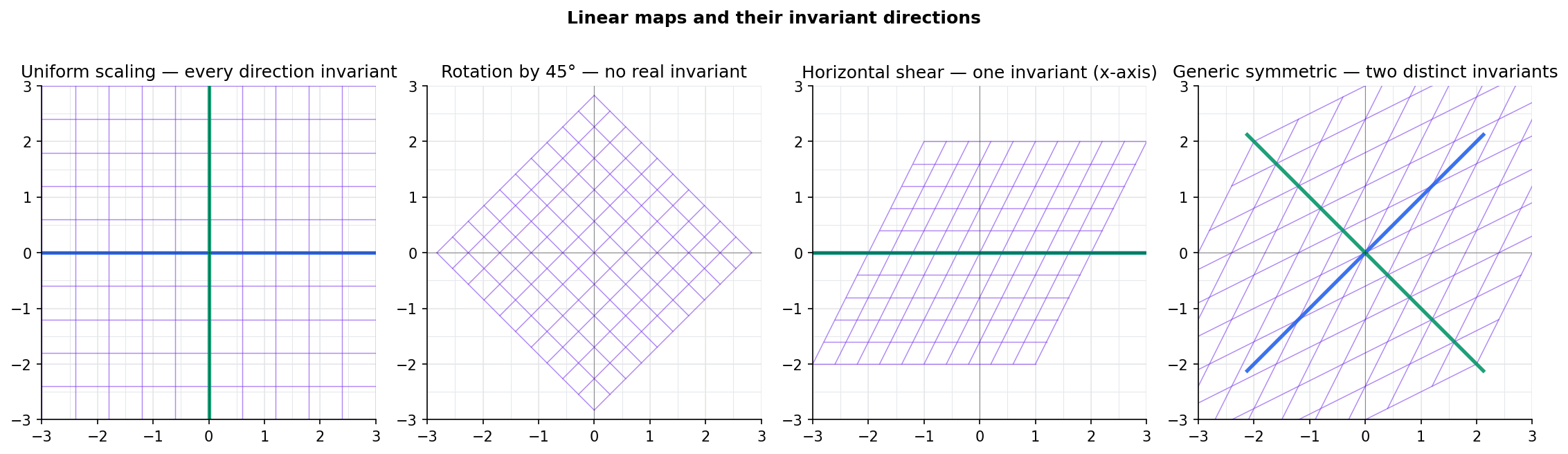
Three maps, three answers: all, none, one. A generic matrix turns out to have two invariant directions, not three, not one. The question of how many invariant directions a linear map has — and which — is itself nontrivial, and the rest of this topic is the systematic theory that answers it.
We can write the question as a single equation. A nonzero vector lies along an invariant direction of exactly when is parallel to — that is, when is some scalar multiple of :
The scalar records how scales the vector along the invariant direction. For the uniform scaling, for every direction. For the rotation, no real works for any nonzero real . For the shear, for the -axis. This single equation — three symbols on the left, three on the right — is the rest of the topic in concentrated form.
ML aside. When a paper says “the dominant eigenvector of the Hessian points in the direction of largest curvature,” the noun eigenvector is the object this section is about to name: a direction the matrix doesn’t rotate, only stretches. The factor by which it stretches is the eigenvalue — the curvature in that direction. The Hessian topic invoked this picture without justification; this topic justifies it.
The viz below lets you build a matrix one entry at a time and see the invariant directions appear in real time. Drag the matrix entries, watch the eigenvectors slide around, and notice which preset matrices have zero, one, or two real invariant directions. The defective Jordan block and the rotation preset are the two cases where the eigenvector story is more interesting than “two distinct lines” — they motivate §5 (defective matrices) and §3 (complex eigenvalues), respectively.
- λ = 3.00
- λ = 2.00
- v = (0.89, 0.45) for λ = 3.00
- v = (0.71, 0.71) for λ = 2.00
2. Eigenvalues, Eigenvectors, and Eigenspaces
The verbal question of §1 — which directions does a linear map merely scale? — becomes precise once we name the objects. A nonzero vector that gets only scaled is an eigenvector; the scaling factor is the eigenvalue; the set of all eigenvectors for a fixed eigenvalue, together with the zero vector, is the eigenspace. These three pieces of vocabulary will recur in every section below.
📐 Definition 1 (Eigenvalue, Eigenvector, Eigenspace)
Let be a real vector space and a linear map. A nonzero vector is an eigenvector of with eigenvalue (or , when we work in the complex setting) if
The set
is the eigenspace of corresponding to . The set of all eigenvalues of is the spectrum, written .
A few features of the definition deserve immediate comment. First, the equation is homogeneous of degree one in : if is an eigenvector with eigenvalue , so is for any nonzero scalar — eigenvectors come in lines through the origin, not as isolated vectors. Second, the eigenvalue is determined by the eigenvector (apply , see how much it scales), but a single eigenvalue may have many eigenvectors — every nonzero element of is an eigenvector for . Third, although the definition is stated for an abstract linear map, in practice we will work with a fixed basis and identify with its matrix ; the equation becomes , and the eigenvectors and eigenvalues are properties of the matrix.
🔷 Proposition 1 (Eigenspaces Are Subspaces)
For any linear map and any scalar , the eigenspace is a subspace of . In particular, contains the zero vector and is closed under addition and scalar multiplication.
Proof.
Rewrite the eigenspace as , where is the linear map . To see the rewrite: if and only if , which is equivalent to , which is the statement . The kernel of any linear map is a subspace (Proposition 2 of Linear Algebra), so is a subspace.
Concretely: the zero vector satisfies , so . If , then , so . Scalar multiplication is analogous.
The eigenspace is a subspace, so it has a dimension; that number measures the “size” of the invariant direction (a line, a plane, all of ) corresponding to .
📐 Definition 2 (Geometric Multiplicity)
The geometric multiplicity of an eigenvalue of is the dimension of its eigenspace:
For any actual eigenvalue , the eigenspace contains at least one nonzero eigenvector, so .
Three running examples will be referenced throughout the topic; each shows a different qualitative behavior of the eigenvalue equation.
📝 Example 1 (A diagonal matrix)
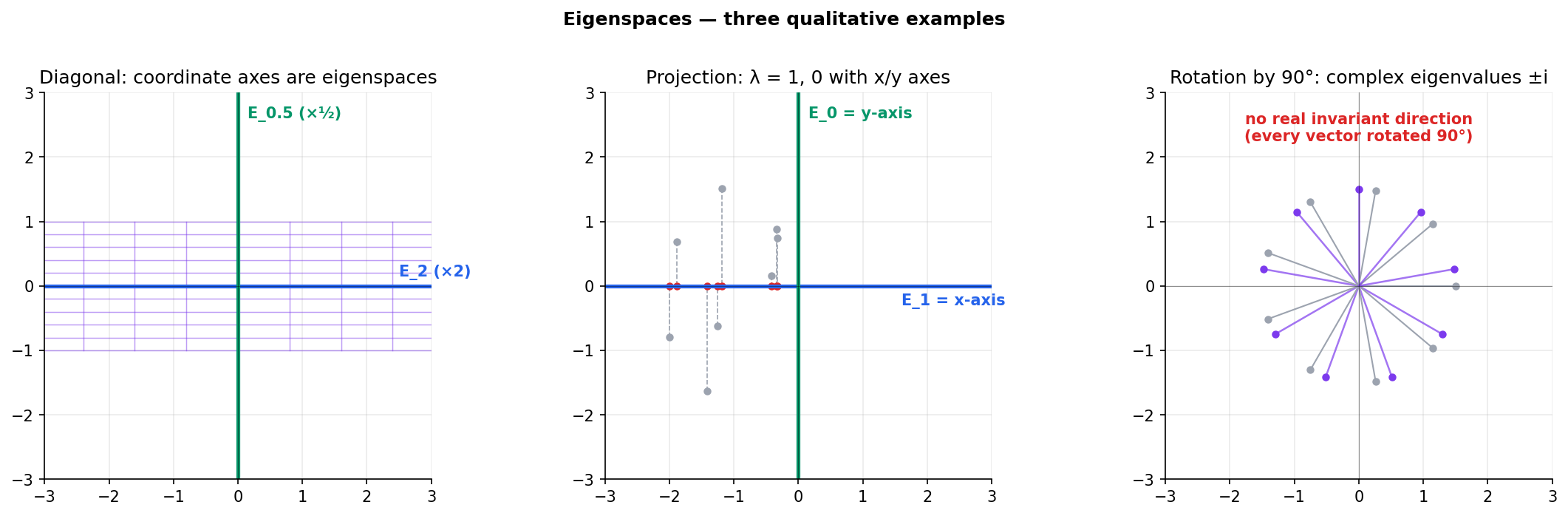
Let — the matrix with on the diagonal and zeros elsewhere. For each standard-basis vector , direct computation gives . So is an eigenvector with eigenvalue for every . The eigenvalues are exactly the diagonal entries (with their multiplicities), and the eigenspaces are the coordinate axes — or sums of coordinate axes, when entries are repeated. A diagonal matrix is the easiest possible eigenvalue picture: the standard basis is already an eigenbasis.
📝 Example 2 (A projection)
Let be orthogonal projection onto the -axis: . Then and . The eigenvectors are with eigenvalue and with eigenvalue . The eigenspace is the -axis (vectors that the projection leaves untouched), and is the -axis (vectors that the projection collapses to the origin). The map is fully described by the data “stretch by along the -axis, kill the -axis” — and that data is exactly the eigenvalue / eigenspace pair. Example 15 of Linear Algebra used this projection to motivate change of basis; here it reappears as the prototypical eigenvalue example.
📝 Example 3 (Rotation by π/2)
Let be rotation by counterclockwise: , with matrix . No nonzero real vector is fixed up to scaling by a rotation — every direction is mapped to the perpendicular direction, never to a scalar multiple of itself. So has no real eigenvalues at all.
Over the complex numbers, the situation changes. Try the candidate : , so is a complex eigenvector with eigenvalue . The conjugate is an eigenvector with eigenvalue . Real matrices can have complex eigenvalues — and when they do, the eigenvalues come in complex conjugate pairs. The real-vs-complex distinction will return in §3 when we develop the characteristic polynomial.
The three examples already span the qualitative behaviors we will need to organize: every direction invariant (Example 1 with ), exactly two directions invariant (Example 2, and generic matrices), and no real direction invariant (Example 3). The first nontrivial structural fact about eigenvectors — the one that drives diagonalizability in §4 — is that eigenvectors for distinct eigenvalues cannot be linearly dependent.
🔷 Proposition 2 (Distinct Eigenvalues Imply Independent Eigenvectors)
Let be a linear map and let be eigenvectors of with eigenvalues . If the eigenvalues are pairwise distinct, then the eigenvectors are linearly independent.
Proof.
We induct on . For , the claim is just , which is part of the definition of eigenvector.
For the induction step, assume the result for any eigenvectors with distinct eigenvalues, and suppose
for some scalars . Apply to both sides. Since is linear and each is an eigenvector with eigenvalue ,
Now multiply by and subtract from to eliminate the term:
The first eigenvectors have pairwise distinct eigenvalues (since all are pairwise distinct), so by the inductive hypothesis they are linearly independent. Each coefficient must therefore vanish:
Since , we conclude for . Plugging back into leaves , and since , as well. So every vanishes — the eigenvectors are linearly independent.
🔷 Corollary 1 (At most dim V distinct eigenvalues)
A linear map on a finite-dimensional vector space has at most distinct eigenvalues.
Proof.
A linearly independent set in has at most elements (Proposition 5 of Linear Algebra). Choose one eigenvector from each distinct eigenvalue: by Proposition 2, the resulting list is linearly independent, so its length — the number of distinct eigenvalues — is at most .
The corollary is the structural ceiling that makes diagonalization possible. If a matrix has three distinct eigenvalues, we automatically get three linearly independent eigenvectors — and by §4, that means we can change basis to make the matrix diagonal. Repeated eigenvalues may still allow a basis of eigenvectors (Example 1 with and the scalar matrix are textbook cases) but the guarantee comes only with distinctness.
💡 Remark 1 (Why we exclude the zero vector)
The definition insists that for an eigenvector. The reason is bookkeeping: if we allowed , then would hold for every scalar . The zero vector would be an “eigenvector for every eigenvalue,” and the notion of “the eigenvalue of ” would be meaningless. By excluding it, each eigenvector pins down a unique eigenvalue, and the eigenvalue equation becomes a constraint on the direction of rather than a triviality. Note that the eigenspace does contain — otherwise it would not be a subspace — but is not itself called an eigenvector.
ML aside. When you decompose a weight matrix as (the singular value decomposition, which we will not develop here), the are not eigenvalues of — they are eigenvalues of , which is symmetric and therefore covered by the spectral theorem in §6. The eigenvalues of itself are typically complex and less useful in ML practice. The reason the symmetric case dominates ML applications is that the matrices that actually matter (covariance, Hessian, , kernel Gram) are all symmetric. The symmetric story is the headline of this topic; the general case (§§3–5) is the warm-up that prepares it.
3. The Characteristic Polynomial
Definition 1 names the eigenvalue equation , but it does not yet tell us how to find the eigenvalues of a given matrix. The bridge from “what is an eigenvalue?” to “compute the eigenvalues” is the characteristic polynomial: a single polynomial in one variable whose roots are exactly the eigenvalues, and whose degree is the dimension of the underlying space.
The construction starts with a rewriting of the eigenvalue equation. The condition is the same as , which is the same as . So is a nonzero element of . By the invertibility characterization of Linear Algebra (Corollary 1 of §8), a square matrix is non-invertible exactly when its determinant is zero. Therefore is an eigenvalue if and only if — which is a single equation in the single variable .
📐 Definition 3 (Characteristic Polynomial)
For an matrix , the characteristic polynomial of is
It is a monic polynomial in of degree with real coefficients (assuming is real). The characteristic equation is .
🔷 Theorem 1 (Eigenvalues Are Roots of the Characteristic Polynomial)
For any matrix and any scalar :
Proof.
is an eigenvalue of iff there exists a nonzero with , i.e. . By the invertibility characterization (Corollary 1 of §8 of Linear Algebra), this is equivalent to being non-invertible, which is equivalent to .
Finally, — multiplying every row of a matrix by multiplies the determinant by — so the two determinants vanish together. Therefore if and only if is an eigenvalue.
Theorem 1 changes the entire character of the eigenvalue problem. We no longer have to guess eigenvalues — we compute them by finding roots of a polynomial. The polynomial has degree , so by the Fundamental Theorem of Algebra it has exactly roots over , counted with multiplicity. A real matrix therefore has exactly eigenvalues over the complex numbers, though fewer may be real.
📐 Definition 4 (Algebraic Multiplicity)
The algebraic multiplicity of an eigenvalue of is its multiplicity as a root of the characteristic polynomial: the largest integer such that divides when is the eigenvalue in question. We write for this number.
A natural question follows immediately. We have two notions of “multiplicity” for an eigenvalue: the geometric one (Definition 2, the dimension of ) and the algebraic one we just named. How do they relate? The answer is that geometric multiplicity is bounded above by algebraic multiplicity, and the gap between them is the source of all the eigenvalue pathology to come.
🔷 Proposition 3 (Geometric ≤ Algebraic Multiplicity)
For any eigenvalue of , the geometric multiplicity is at most the algebraic multiplicity:
Proof.
Let be the geometric multiplicity. Choose a basis of the eigenspace , and extend it to a basis of (using the basis-extension lemma from §3 of Linear Algebra). In this basis, the matrix of has block form
for some block and block . The reason: for each , so the first columns of are times the corresponding standard basis vectors. The bottom-left block is zero because the eigenvectors have no components. The remaining columns are arbitrary, filling out the blocks and .
Similar matrices share the characteristic polynomial (Lemma 1 below), so
using the block-triangular determinant formula. The factor contributes at least to the multiplicity of as a root, so .
The proof used a fact we now make explicit: similar matrices have the same characteristic polynomial. The intuition is that similarity corresponds to a change of basis, and the characteristic polynomial is a property of the underlying linear map — not of the matrix that happens to represent it in a particular basis.
🔶 Lemma 1 (Similar Matrices Have the Same Characteristic Polynomial)
If and are similar — meaning for some invertible — then .
Proof.
Using the multiplicativity of the determinant (Theorem 6 of Linear Algebra) and :
Pulling the determinants apart and rearranging gives
So .
In particular, and have the same eigenvalue multiset (with algebraic multiplicities), the same trace (sum of eigenvalues), and the same determinant (product of eigenvalues) — all because the characteristic polynomial is a similarity invariant.
The next examples compute for small matrices and illustrate the three qualitatively different scenarios: distinct real roots, a repeated real root, and a complex conjugate pair.
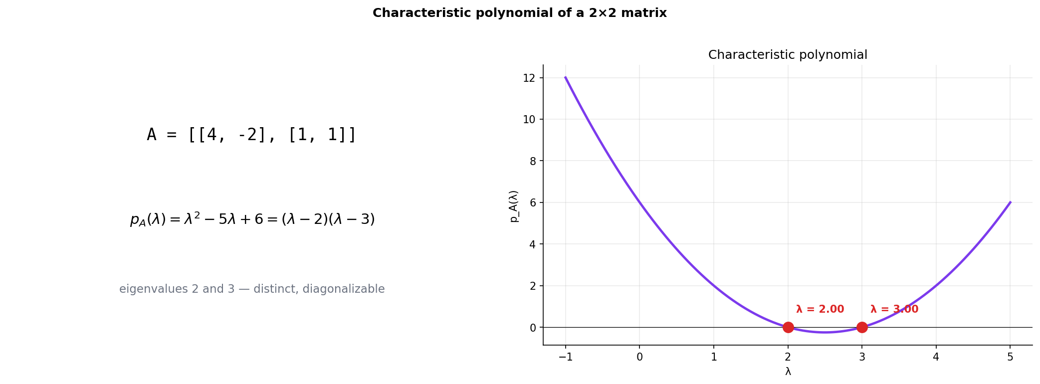
📝 Example 4 (Characteristic polynomial of a 2×2 matrix)
For :
The coefficients are familiar: and , so
Solving the quadratic gives the eigenvalues
Apply to : , , so . Eigenvalues , .
📝 Example 5 (A 2×2 matrix with complex eigenvalues)
For the 90° rotation from Example 3: , , so . The roots are — no real eigenvalues. Over the complex numbers the eigenvectors are and . A real matrix can have complex eigenvalues; when it does, they come in complex conjugate pairs (because the characteristic polynomial has real coefficients, so non-real roots arise in conjugate pairs).
📝 Example 6 (A 3×3 characteristic polynomial)
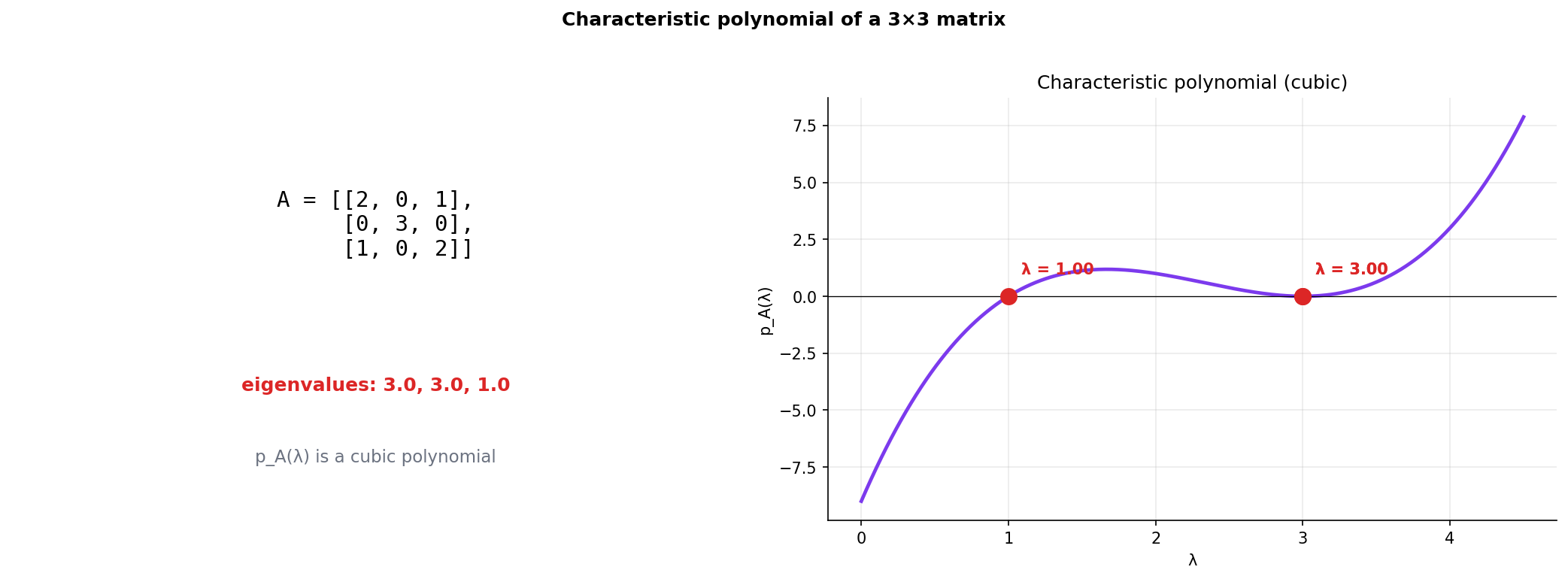
For — upper-triangular, so the characteristic polynomial factors immediately:
Eigenvalues: with algebraic multiplicity 2 and with algebraic multiplicity 1. Whether ‘s geometric multiplicity is 1 or 2 depends on the off-diagonal entries — this matrix happens to be defective (geometric multiplicity 1), so it is not diagonalizable. We return to this in §5.
💡 Remark 2 (Real vs. complex eigenvalues)
Over the real numbers, a polynomial of degree may have fewer than real roots: as Example 5 showed, has no real roots even though its degree is 2. The Fundamental Theorem of Algebra guarantees that over the complex numbers, every degree- polynomial has exactly roots counted with multiplicity. So a real matrix always has complex eigenvalues (with multiplicity), but possibly fewer real ones.
Real eigenvalues correspond to invariant directions in the geometric sense of §1 — directions the map stretches without rotating. Complex eigenvalues correspond to rotational behavior: when is complex, the action of on the real 2-plane spanned by the real and imaginary parts of the complex eigenvector is a rotation by angle combined with a scaling by . The 90° rotation in Example 5 has (pure rotation, no scaling) and angle . Real symmetric matrices — the headline case of §6 — never have complex eigenvalues, because their characteristic polynomials factor over the reals.
💡 Remark 3 (Computational reality)
Computing eigenvalues by writing down and factoring it works fine for and and is unusable for . Wilkinson’s polynomial — the characteristic polynomial of a deliberately constructed matrix — is so ill-conditioned that floating-point errors of order in the coefficients move the roots by order 1. Even for benign-looking matrices, the polynomial coefficients accumulate cancellation error and the roots become hopelessly inaccurate.
Production eigenvalue solvers use the QR algorithm (Francis, 1961) — an iterative orthogonal-similarity transformation that converges to a Schur form, from which eigenvalues read off the diagonal — and the Lanczos / Arnoldi iterations for sparse matrices when only a few extremal eigenvalues are needed. Both algorithms bypass the characteristic polynomial entirely. We cite this without developing the numerical theory; Trefethen & Bau, Numerical Linear Algebra (Lectures 24–30) is the right reference. The notebook for this topic uses np.linalg.eig and np.linalg.eigh for matrices larger than — and so, in practice, do you.
ML aside. When the Hessian topic spoke of “the eigenvalues of ,” it implicitly used the characteristic polynomial to define them. For low-dimensional examples (e.g., a Hessian of a 2-feature regression), you can write and solve. For real ML problems with for in the millions, the characteristic polynomial is unreachable, and practitioners use truncated iterative methods (Lanczos for the top- eigenvalues of a sparse PSD Hessian) to extract just the eigenvalues that matter — typically the largest few (governing the loss landscape’s dominant curvatures) and the smallest few (governing convergence-limiting slow modes).
The viz below plots as a curve in the plane for a user-controlled or matrix. Real eigenvalues appear as filled circles where the curve crosses zero; complex roots appear in an inset Argand plane.
- λ = 3.00
- λ = 2.00
4. Diagonalizability and Similarity
The characteristic polynomial tells us how many eigenvalues a matrix has and what they are. The next question is whether the eigenvectors form a basis of — because when they do, the matrix becomes diagonal in that basis, and most calculations involving the matrix (powers, exponentials, system solutions) collapse to trivial scalar arithmetic along the eigenbasis.
📐 Definition 5 (Diagonalizable Matrix)
An matrix is diagonalizable (over the field , typically or ) if there exists an invertible and a diagonal matrix — both with entries in — such that
Equivalently, is similar to a diagonal matrix.
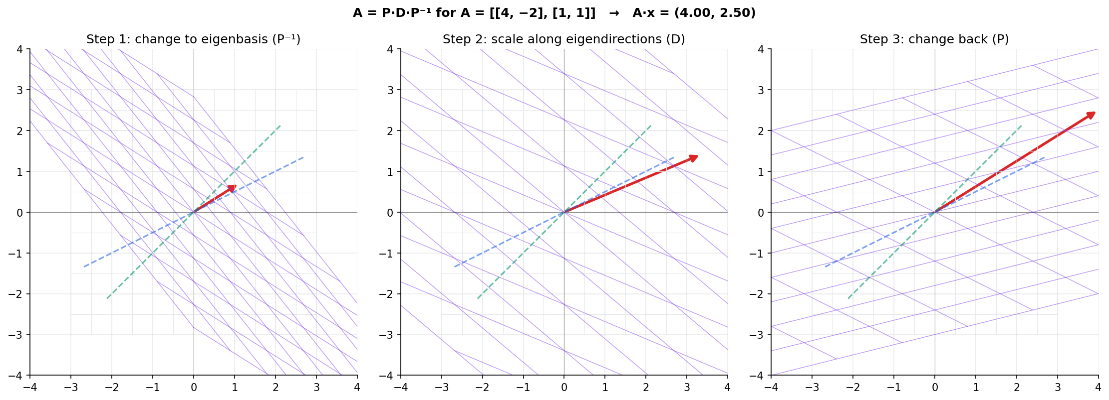
The factorization is the eigendecomposition. Geometrically: change of basis to the eigenbasis (apply ), scale along each eigendirection independently (apply ), change back to the standard basis (apply ). Algebraically: every action of on a vector reduces to independent scalar scalings in the eigenbasis.
🔷 Theorem 2 (Diagonalizability and Eigenbases)
An matrix is diagonalizable if and only if there exists a basis of (or , depending on the field) consisting of eigenvectors of . In that case, the columns of are the eigenvectors, and the diagonal entries of are the corresponding eigenvalues.
Proof.
() Suppose with and invertible with columns . Multiply both sides on the right by to clear the inverse: . Reading column of both sides: . So each column of is an eigenvector with eigenvalue equal to the corresponding diagonal entry of . Since is invertible, its columns are linearly independent, hence a basis of .
() Suppose is a basis of eigenvectors with eigenvalues . Form the matrix whose columns are these eigenvectors; is invertible because its columns are linearly independent. Form . Then by column-by-column computation (each column of is , and each column of is ). Multiply both sides on the right by to conclude .
The most useful immediate consequence is that distinct eigenvalues are enough to guarantee diagonalizability. We never have to check geometric vs. algebraic multiplicities for distinct-eigenvalue matrices.
🔷 Corollary 2 (Distinct Eigenvalues Imply Diagonalizable)
If an matrix has distinct eigenvalues (each with algebraic multiplicity 1), then is diagonalizable.
Proof.
Pick one eigenvector from each eigenspace . By Proposition 2 (§2), eigenvectors for distinct eigenvalues are linearly independent. So is a list of linearly independent vectors in , hence a basis. By Theorem 2, is diagonalizable.
For repeated eigenvalues, diagonalizability is no longer automatic. The criterion is multiplicity-by-multiplicity equality: every repeated eigenvalue must have a geometric multiplicity that matches its algebraic multiplicity.
🔷 Theorem 3 (Diagonalizability Criterion via Multiplicities)
An matrix is diagonalizable (over a field containing all its eigenvalues) if and only if, for every eigenvalue , the geometric multiplicity equals the algebraic multiplicity:
Proof.
() Suppose for every eigenvalue. The eigenspaces for distinct eigenvalues are linearly independent subspaces (extending Proposition 2 from single eigenvectors to whole eigenspaces — the same induction works with bases of in place of single vectors). The total dimension of the direct sum is
so the eigenspaces span all of (assuming the field contains all the eigenvalues). Concatenating bases of each eigenspace gives a basis of consisting of eigenvectors; by Theorem 2, is diagonalizable.
() Suppose with . The eigenspace in this representation is the span of the standard basis vectors for which — so equals the count of diagonal entries equal to . The characteristic polynomial is (the diagonal makes this immediate), so is also the count of diagonal entries equal to . The two counts agree.
📝 Example 7 (Diagonalization of a 2×2 matrix)
Continue with . Eigenvalues and (Example 4) — distinct, so is diagonalizable by Corollary 2. Find eigenvectors:
- For : solve , i.e. . The kernel is spanned by .
- For : solve , i.e. . The kernel is spanned by .
Form and . Verify by direct multiplication that . Then where . In the eigenbasis, is the pair of independent scalings — by 3 along and by 2 along .
When two matrices represent the same linear map in different bases, they are similar — and similarity preserves every invariant of the underlying map. The list of similarity invariants is exactly the data we can read off from the eigenvalue picture.
🔷 Theorem 4 (Similarity Invariants)
If and are similar matrices, they share:
(a) the characteristic polynomial (and hence the eigenvalue multiset with algebraic multiplicities),
(b) the trace,
(c) the determinant,
(d) the rank,
(e) the nullity,
(f) the geometric multiplicity of each eigenvalue.
Proof.
(a) is Lemma 1 (§3). (b) Trace equals minus the coefficient of in (this is the elementary-symmetric-polynomial identity), so trace is determined by the characteristic polynomial, hence invariant. (c) Determinant equals times the constant term of , so it too is determined by the characteristic polynomial. (d) The column space of has the same dimension as the column space of : on the right doesn’t change dimension (it’s a bijection from to itself), and on the left maps the column space isomorphically. So rank is preserved. (e) Nullity equals , so it follows from (d) by rank-nullity. (f) The geometric multiplicity of is
the same in both bases.
💡 Remark 4 (Powers and exponentials via diagonalization)
For diagonalizable with :
The pairs telescope. The same identity holds for any function defined on the spectrum:
In particular,
This is the spectral mapping observation: functions of a diagonalizable matrix are computed by applying the function to the diagonal of , then sandwich-wrapping. Closed-form matrix exponentials, square roots of positive-definite matrices, and whitening transformations are all instances.
ML aside. When the Linear Systems topic wrote for the solution of , it was applying exactly Remark 4. The matrix exponential of a diagonalizable matrix reduces to independent scalar exponentials along the eigenbasis. The continuous-time gradient flow has solution , and each eigencomponent decays independently. The eigenbasis is the basis in which the dynamics decouple — that is the actual reason eigenvalues control convergence.
   0.89    0.71
   0.45    0.71
   3.00    0.00
   0.00    2.00
   2.24   -2.24
  -1.41    2.83
5. Defective Matrices — A Brief Detour
Not every matrix is diagonalizable. When an eigenvalue’s algebraic multiplicity strictly exceeds its geometric multiplicity — the eigenspace is “smaller than it should be” — the matrix is called defective. The defective case is structurally important enough to name and exhibit, but the full theory of canonical forms for defective matrices (Jordan canonical form) is mathematically heavy and rarely needed in ML practice. We name the form, give one example, and forward the full development to a future topic.
📐 Definition 6 (Defective Matrix)
An matrix is defective if it has an eigenvalue whose geometric multiplicity is strictly less than its algebraic multiplicity. Equivalently, has fewer than linearly independent eigenvectors, so it admits no eigenbasis and is not diagonalizable.
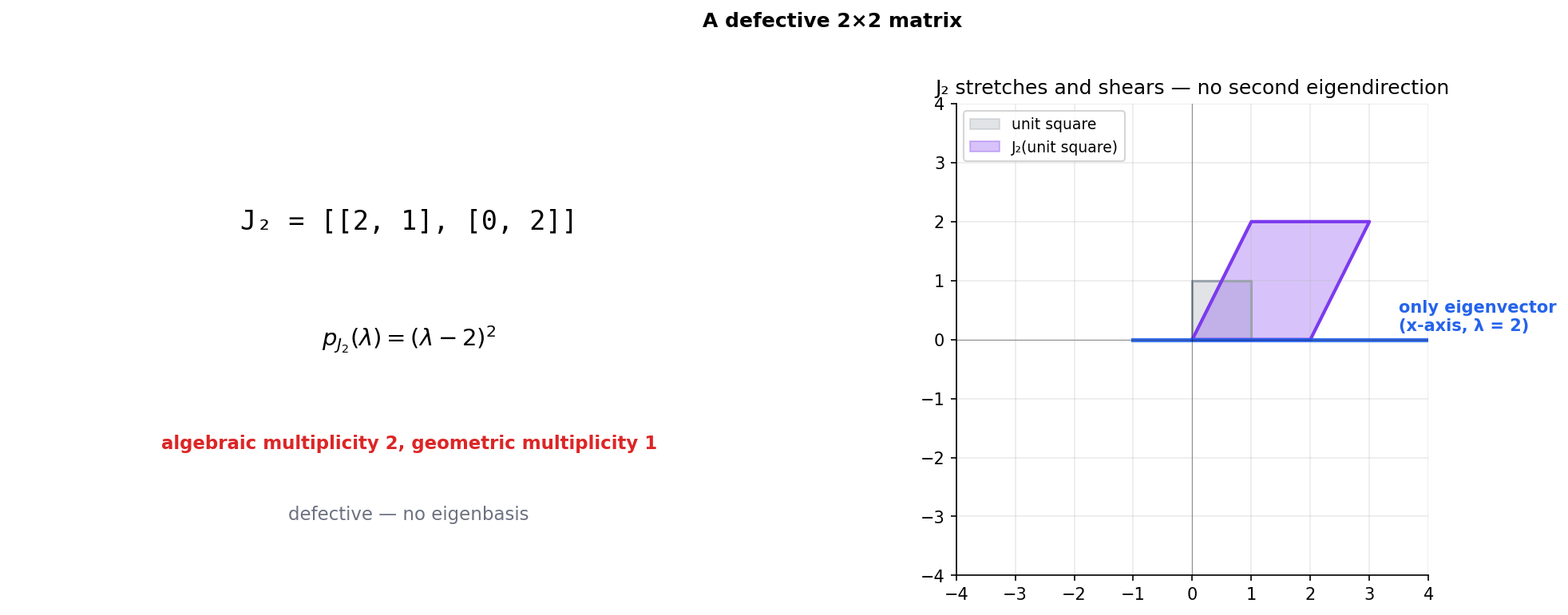
📝 Example 8 (A defective 2×2 matrix)
Let . Characteristic polynomial: . So is the only eigenvalue, with algebraic multiplicity 2.
Compute the eigenspace by solving :
The eigenspace is one-dimensional. Geometric multiplicity 1, algebraic multiplicity 2: is defective. There is no basis of consisting of eigenvectors of , so is not diagonalizable. The matrix is already in Jordan form — it is a Jordan block.
📐 Definition 7 (Jordan Block (informal))
A Jordan block of size with eigenvalue is the matrix
with on the diagonal, s on the immediate superdiagonal, and s elsewhere. The matrix in Example 8 is the Jordan block of size 2 with eigenvalue 2.
🔷 Theorem 5 (Jordan Canonical Form (stated, not proved))
Every matrix over the complex numbers is similar to a block-diagonal matrix whose blocks are Jordan blocks . The list of Jordan blocks — their sizes and eigenvalues — is unique up to ordering, and is the Jordan canonical form of . The Jordan form is the canonical generalization of diagonalization: diagonalizable matrices are exactly those whose Jordan form has all blocks.
💡 Remark 5 (Why we don't develop Jordan form)
The proof of Theorem 5 (see Hoffman-Kunze Chapter 7 or Horn-Johnson Chapter 3) requires generalized eigenvectors, Jordan chains, and a careful induction on the algebraic multiplicity of each eigenvalue. The development is mathematically beautiful but long, and the practical payoff is modest: defective matrices are rare in clean applications, and when they do arise (linear-systems repeated eigenvalues, bifurcation analysis), the relevant techniques can be developed locally on a case-by-case basis.
We treat Linear Systems & Matrix Exponential as the place where case-by-case handling for defective systems lives; the full Jordan theory belongs to a future topic on canonical forms or numerical linear algebra. For the rest of this topic, we proceed as if all matrices are diagonalizable — a working assumption that holds for the symmetric matrices §6 puts at the center, and for generic random matrices in general.
💡 Remark 6 (Defective matrices are measure-zero but not negligible)
The set of matrices with all distinct eigenvalues is open and dense in the space of all matrices ; its complement, where some eigenvalues coincide, is a set of measure zero (the discriminant of the characteristic polynomial vanishes on a hypersurface). So a random matrix is diagonalizable with probability 1.
But defective matrices live on the boundary between qualitatively different behaviors — e.g. the boundary between a stable spiral and a stable node in a 2D phase portrait, or the boundary between under-damped and over-damped oscillation in a second-order linear system. Bifurcation theory studies exactly what happens at such boundaries, and there defectiveness is the central object, not an exception. ML reality: repeated eigenvalues of the Hessian at a critical point are a measure-zero coincidence in a generic loss landscape, but at symmetric critical points (e.g. loss invariant under permutation of neurons in a wide network) they become structural rather than accidental.
6. Symmetric Matrices and the Spectral Theorem
The defective case in §5 is the bad news about the general eigenvalue picture. The good news is that the matrices ML actually cares about — the Hessian of a smooth loss, the covariance of a random vector, the Gram matrix , the kernel Gram, the graph Laplacian — are all symmetric. And real symmetric matrices have the cleanest possible eigenvalue behavior: real eigenvalues, orthogonal eigenvectors, always diagonalizable, and a factorization where is orthogonal and is diagonal-real. This is the spectral theorem, the centerpiece of the topic.
📐 Definition 8 (Symmetric Matrix)
A real matrix is symmetric if , i.e. for every pair of indices .
Three structural facts about symmetric matrices, in increasing order of strength: all eigenvalues are real (Lemma 2), eigenvectors for distinct eigenvalues are automatically orthogonal (Lemma 3), and the eigenspaces span all of — so a symmetric matrix always has an orthonormal eigenbasis (Theorem 6). Each fact’s proof is a short computation; together they give the spectral theorem.
🔶 Lemma 2 (Symmetric Matrices Have Real Eigenvalues)
Every eigenvalue of a real symmetric matrix is real.
Proof.
Let be an eigenvalue of the real symmetric matrix , with a corresponding (possibly complex) eigenvector : .
Take the conjugate transpose (, ): . Since is real and symmetric, . So .
Multiply the eigenvalue equation on the left by : . Multiply on the right by : .
Equate the two expressions: . Since , . Divide both sides by to get , hence .
🔶 Lemma 3 (Symmetric Matrices Have Orthogonal Eigenspaces)
If is real symmetric and are eigenvectors of corresponding to distinct eigenvalues , then .
Proof.
Compute two ways. First, using :
Second, pushing the across the inner product using (a property of the symmetric case, see §10 of Linear Algebra on inner products and adjoints):
Equating: , i.e. . Since , the inner product .
With both lemmas in hand, the spectral theorem is the inductive payoff. The structure of the proof is the heart of the topic: find one eigenvalue/eigenvector pair using Lemma 2, peel off its 1-dimensional eigenspace, and recurse on the -dimensional orthogonal complement — which remains symmetric.
🔷 Theorem 6 (Spectral Theorem for Real Symmetric Matrices)
Let be a real symmetric matrix. Then there exists an orthogonal matrix (i.e. ) and a real diagonal matrix such that
The columns of form an orthonormal basis of consisting of eigenvectors of ; the diagonal entries of are the corresponding eigenvalues (with algebraic multiplicities, conventionally listed in non-increasing order ).
Proof.
Induction on .
Base case (). A matrix is trivially symmetric and diagonal: take and .
Inductive step. Assume the spectral theorem holds for symmetric matrices. Let be an real symmetric matrix.
By Lemma 2, the characteristic polynomial has at least one real root (in fact, all its roots are real, but we only need one for the induction). By Theorem 1, is a real eigenvalue. Pick a corresponding real unit eigenvector with .
Extend to an orthonormal basis of via Gram-Schmidt (§10 of Linear Algebra). Form the orthogonal matrix whose columns are these vectors; orthogonal because the columns are orthonormal.
Consider the matrix . Two things are true about it.
First, it is symmetric: (using ).
Second, its first column equals : the -th column of is \tilde Q^\top A (\text{j-th column of } \tilde Q). For , this is , since by construction (the first column of is ).
Combining symmetry with the first column being forces the first row to be as well. So
for some block . The block is symmetric (symmetry of the full matrix passes to the lower-right block). By the inductive hypothesis, with orthogonal and diagonal real.
Define
Then is orthogonal (block-diagonal with orthogonal blocks) and is diagonal. A direct computation gives . Set — orthogonal as a product of orthogonals. Then , completing the induction.
🔷 Corollary 3 (Spectral Decomposition as a Sum of Rank-One Projectors)
Under the spectral theorem, has the outer-product expansion
where each is the rank-one orthogonal projector onto . The matrix is therefore a weighted sum of rank-one projectors onto its eigendirections, weighted by the eigenvalues.
Proof.
Direct expansion of . The matrix scales the -th row of (which is ) by . Multiplying by on the left forms the outer product .
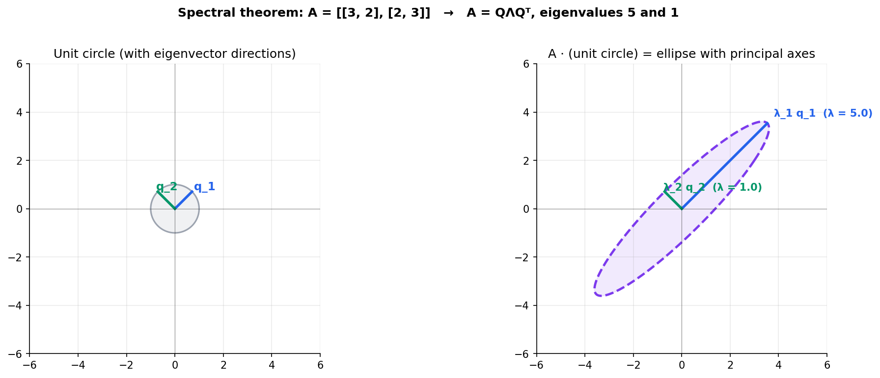
📝 Example 9 (Diagonalizing a 2×2 symmetric matrix)
Let . Trace = 5, determinant = 0. Characteristic polynomial: . Eigenvalues: and .
For : solve , i.e. . The kernel is spanned by ; normalize to .
For : solve . The kernel is spanned by ; normalize to .
Verify orthogonality: ✓, exactly as Lemma 3 promised.
Spectral decomposition: — a rank-one matrix, consistent with . The image of is the line spanned by ; the null space is the line spanned by .
💡 Remark 7 (Why symmetric is so much cleaner)
The proof of Theorem 6 uses no polynomial algebra. It does not factor the characteristic polynomial or count multiplicities. The induction step finds one eigenvalue–eigenvector pair (Lemma 2 guarantees the eigenvalue is real), restricts to the orthogonal complement (which inherits symmetry), and recurses. The argument is purely geometric: find an invariant line, peel it off, repeat. The same argument generalizes verbatim to compact self-adjoint operators on infinite-dimensional Hilbert spaces — the proof in Hilbert Spaces of the infinite-dim spectral theorem is structurally identical to ours.
💡 Remark 8 (Real-symmetric vs. complex-Hermitian)
The complex analogue of a real symmetric matrix is a Hermitian matrix: where . The complex spectral theorem says every Hermitian matrix factors as with unitary () and real diagonal. The proof is structurally identical to ours; only the inner product changes (, conjugate-linear in the first slot). Quantum mechanics lives in this setting — observables are Hermitian operators, and their real eigenvalues are the measurable values. For ML the real symmetric case suffices.
💡 Remark 9 (The Hessian, revisited)
Recall from the Hessian topic that the Hessian of a function is symmetric (Clairaut’s theorem). The spectral theorem now applies: with real eigenvalues. The principal curvatures of the loss surface in the directions are exactly the eigenvalues . The second-derivative test reads off the critical-point type from the signs of the : all positive ⟹ local minimum, all negative ⟹ local maximum, mixed signs ⟹ saddle. We now have the rigorous spectral foundation for that test; §7 makes it formal as Theorem 7.
ML aside. A covariance matrix is symmetric by construction (the outer-product structure forces ). The spectral theorem gives with orthogonal and diagonal-real-non-negative. The columns of are the principal components of the distribution; the diagonal entries of are the variances along those directions. PCA is literally the spectral theorem applied to a covariance matrix. The whitening transformation (well-defined when is positive-definite) maps the distribution to one with identity covariance — the precondition for Mahalanobis distance and for well-conditioned gradient descent. multivariate-distributions → pca-and-spectral-methods →
7. Quadratic Forms and Positive-Definiteness
The spectral theorem unlocks the classification of quadratic forms — scalar functions of the form with symmetric. In the eigenbasis, becomes spectacularly simple: where are the coordinates of in the eigenbasis. The sign and growth behavior of are then entirely determined by the signs of the eigenvalues. This is the framework in which every convexity statement, every second-derivative test, and every covariance-matrix property on the rest of the site is phrased.
📐 Definition 9 (Quadratic Form)
A quadratic form on is a function of the form for some symmetric matrix . (Any matrix in can be replaced by its symmetric part without changing the form, so we may take symmetric without loss of generality.)
📐 Definition 10 (Definiteness)
A symmetric matrix is
- positive-definite (written ) if for every ;
- positive-semidefinite (written ) if for every ;
- negative-definite if ;
- negative-semidefinite if ;
- indefinite if takes both positive and negative values.
🔷 Theorem 7 (Definiteness via Eigenvalues)
A symmetric matrix is positive-definite iff all eigenvalues are strictly positive; positive-semidefinite iff all eigenvalues are non-negative; negative-definite iff all eigenvalues are strictly negative; indefinite iff it has both positive and negative eigenvalues.
Proof.
By the spectral theorem, with orthogonal and . Substitute :
Since is orthogonal, the map is a bijection, and iff . The form is strictly positive for every iff every (because we can choose to isolate ). Non-negativity, negativity, etc. follow analogously. Indefiniteness corresponds to mixed eigenvalue signs because choosing for the positive eigenvalue makes the form positive, and for the negative eigenvalue makes it negative.
🔷 Corollary 4 (Positive-Definite Matrices Are Invertible)
If , then , so is invertible. The inverse is also positive-definite, with eigenvalues .
🔷 Theorem 8 (Sylvester's Criterion)
A symmetric matrix is positive-definite iff all leading principal minors — the determinants of the upper-left submatrices, for — are strictly positive.
Proof.
() If , then for any nonzero , the extended vector satisfies where is the leading submatrix. Since and , this is positive; so as well, hence by Corollary 4.
() The converse uses induction on : the LDLᵀ decomposition with all positive diagonal entries can be built incrementally from the leading principal minors. The full argument is in Horn & Johnson Theorem 7.2.5; the key idea is that positive leading minors force the pivots in symmetric Gaussian elimination to remain positive, which is equivalent to positive-definiteness.
📐 Definition 11 (Ellipsoid)
Let be symmetric positive-definite. The unit ellipsoid of is
By the spectral theorem, is centered at the origin with principal axes along the eigenvectors and semi-axis lengths . Larger eigenvalues give shorter semi-axes — the matrix “stretches more aggressively” along high-eigenvalue directions, so the level set is more compressed there.
📝 Example 10 (Three quadratic forms in ℝ²)
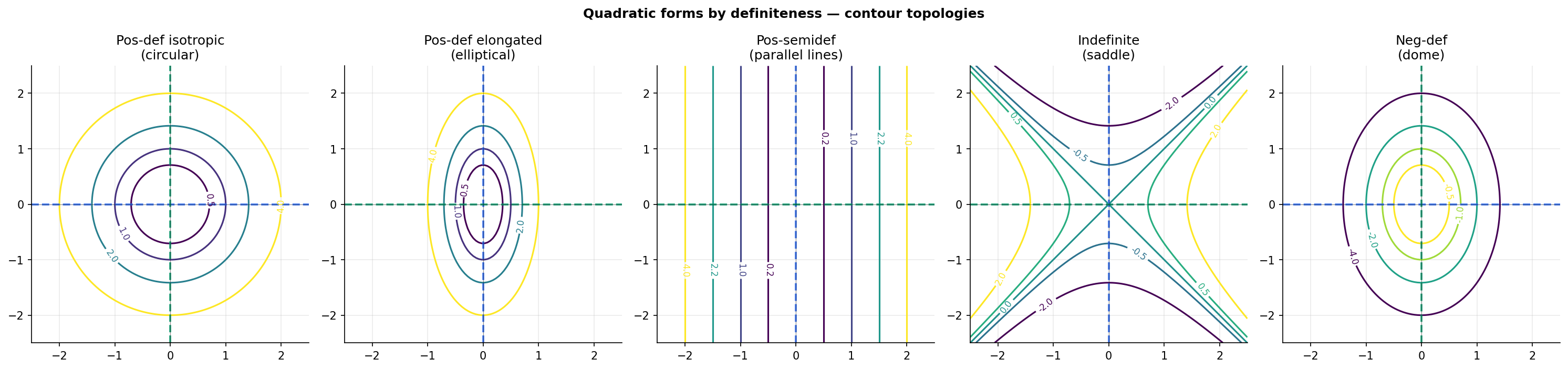
(a) . . Eigenvalues . Level sets are circles of radius . Positive-definite, isotropic.
(b) . . Eigenvalues . Level sets are ellipses with -semi-axis and -semi-axis — elongated along the -axis (smaller eigenvalue, longer axis). Positive-definite, anisotropic.
(c) . . Eigenvalues — opposite signs. The surface is a saddle; level sets are hyperbolas (for ) with asymptotes . Indefinite.
The notebook plots all three. The viz below lets you interpolate continuously between them by editing the matrix entries.
💡 Remark 10 (Why we care about positive-semi-definite (not just positive-definite))
Many naturally occurring symmetric matrices fail to be positive-definite but are positive-semidefinite: a covariance matrix of a degenerate distribution (some linear combination of variables has zero variance); a Gram matrix when the data matrix is rank-deficient; a graph Laplacian, which always has in its kernel. The semidefinite case is where rank-deficiency lives. covariance-correlation → Geometrically, a PSD matrix with a nontrivial kernel has an ellipsoid that degenerates into an infinite cylinder along the kernel direction — the form is constant along the kernel, growing only in the orthogonal complement.
ML aside. The Hessian topic’s “condition number ” implicitly assumes is positive-definite (so ) — that is the local-minimum case. When the Hessian is positive-semidefinite but not positive-definite, the loss has a flat direction (the kernel of ), and gradient descent in that direction is undamped. Modern deep learning has a large literature on flat directions because over-parameterized networks have positive-semidefinite-but-not-positive-definite Hessians by construction (any null direction in parameter space along which the loss does not change is a Hessian-null direction).
8. The Rayleigh Quotient
The spectral theorem and the eigenvalue/definiteness picture (§§6-7) gave us static information about a symmetric matrix: its decomposition, its quadratic form, its principal axes. The Rayleigh quotient gives us a variational characterization — eigenvalues as extrema of a scalar function. This is the picture in which PCA’s “find the direction of maximum variance” lives, and the bridge from spectral theory to constrained optimization.
📐 Definition 12 (Rayleigh Quotient)
For a real symmetric matrix and a nonzero vector , the Rayleigh quotient is
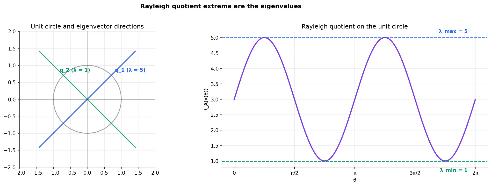
Defined on and scale-invariant: for any . Restricting to unit vectors gives — just the quadratic form on the unit sphere.
🔷 Theorem 9 (Rayleigh Quotient Bounds (Extremal Eigenvalues))
Let be real symmetric with eigenvalues and orthonormal eigenvectors . For every :
The upper bound is achieved at ; the lower bound at . Therefore
Proof.
Expand in the orthonormal eigenbasis: with .
By Parseval (orthonormality of the basis): . By the outer-product expansion (Corollary 3): , so .
Therefore
where are weights summing to . So is a convex combination of the eigenvalues. Any convex combination of numbers lies between the smallest and largest:
Equality on the upper bound requires all the weight to be on indices where — i.e. lies in the eigenspace . The simplest choice is . Similarly the lower bound is achieved at .
🔷 Corollary 5 (Variational Characterization of λ₁ and λₙ)
The maximizer is (top eigenvector); the minimizer is (bottom eigenvector), each up to sign and unit-norm scaling.
📝 Example 11 (Computing λ_max by maximization)
Let . Parameterize the unit circle as . Compute
The maximum over is at (where ); the minimum is at (where ). So , . Top eigenvector , bottom eigenvector .
Sanity-check via the characteristic polynomial: ✓.
💡 Remark 11 (The Rayleigh quotient as a Lagrangian critical-point equation)
The maximization
is a constrained-optimization problem. By Lagrange multipliers (Topic 16), the Lagrangian is
Setting : , i.e. . The Lagrange multiplier at a critical point is an eigenvalue. The critical point is the corresponding eigenvector. Maximizing the Rayleigh quotient is solving the eigenvalue equation — eigenvalues fall out of constrained optimization without any extra machinery.
ML aside. The first principal component of a mean-centered data matrix is the unit vector maximizing — the direction of maximum variance. By Corollary 5, that maximizer is the top eigenvector of , achieving value . Each subsequent component maximizes the same Rayleigh quotient subject to orthogonality with the previous components — exactly the Courant-Fischer characterization of in the next section. PCA is the iterative application of the Rayleigh quotient. pca-and-spectral-methods →
(constrained value, between λmin and λmax)
9. The Courant-Fischer Min-Max Principle
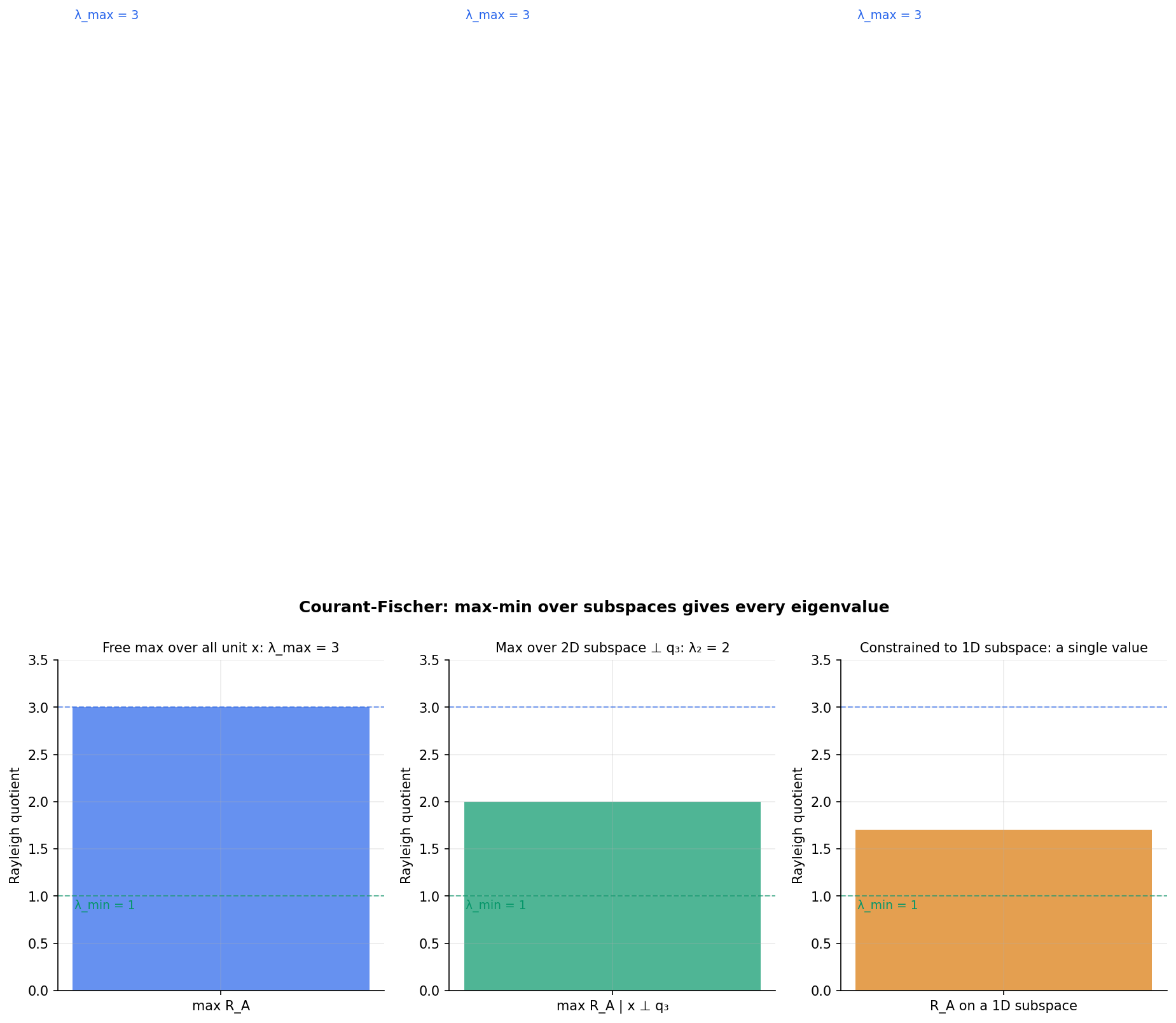
The Rayleigh quotient (§8) characterized and as extrema. What about ? Restricting the Rayleigh quotient to vectors orthogonal to removes the top eigendirection, and the remaining max becomes . But this construction requires already knowing — a chicken-and-egg problem when we want to characterize eigenvalues without first computing the others.
The Courant-Fischer min-max principle avoids the dependence. It characterizes the -th eigenvalue as a max-over--dimensional-subspaces of a min, or equivalently a min-over--dimensional-subspaces of a max. Either formulation captures without first computing .
🔷 Theorem 10 (Courant-Fischer Min-Max Principle)
Let be real symmetric with eigenvalues . For each :
Proof.
We prove the max-min form; the min-max form is the same argument with signs flipped. Let be the orthonormal eigenbasis from the spectral theorem, with and .
Lower bound (). Take , a -dimensional subspace. For any unit with :
since each for . The min over this particular is at least , so the max over all -dim subspaces is at least .
Upper bound (). For any -dimensional subspace , consider its intersection with , an -dimensional subspace. By dimension counting (Topic 33, §8):
So contains a unit vector . Since , expand with . Then
since each for . So for every choice of -dim , the min is at most , and therefore the max over all is at most .
Combining both bounds: .
The Courant-Fischer principle has two important consequences. Cauchy interlacing tells us how eigenvalues of a leading principal submatrix relate to those of the full matrix — a structural fact about how eigenvalues “thin out” as we restrict to subspaces. Weyl’s inequality bounds how much the eigenvalues of a symmetric matrix can move under a perturbation, the foundation of eigenvalue stability in approximate PCA, noise-perturbed kernel methods, and spectral clustering on noisy graphs.
🔷 Corollary 6 (Cauchy Interlacing)
Let be a real symmetric matrix with eigenvalues , and let be the leading principal submatrix of (delete the last row and column). Let be the eigenvalues of . Then
The eigenvalues of interlace those of — between consecutive eigenvalues of .
Proof.
The -dimensional subspaces of embed canonically into as -dimensional subspaces orthogonal to . Apply Courant-Fischer to (working in ) and to (over the same subspaces, restricted to ). The max over a smaller family of subspaces is no larger than the max over the full family, giving . The dual min-max form gives .
🔷 Theorem 11 (Weyl's Inequality (stated))
For real symmetric matrices and of the same size, let denote the -th eigenvalue (in non-increasing order). Then
where is the operator norm. Perturbing by moves each eigenvalue by at most .
💡 Remark 12 (Why Courant-Fischer matters in practice)
Many ML quantities are eigenvalues of matrices that are perturbations of simpler ones — empirical covariance perturbing a population covariance, noisy kernel matrices perturbing the clean kernel, finite-sample graph Laplacians perturbing their continuum limits. Weyl’s inequality (a consequence of Courant-Fischer) says these perturbations move eigenvalues by at most the operator-norm magnitude of the noise — the foundation of eigenvalue stability. The Davis-Kahan theorem extends stability to eigenvectors with sharper conditions; we mention it as the next step in spectral perturbation theory but defer the development.
The min-max characterization also reads as a constrained optimization: “find the best -dimensional approximation of the eigenvalue structure of .” For PCA, this becomes “find the -dim projection that maximizes captured variance” — and Courant-Fischer says the optimal projection is onto the span of the top eigenvectors. Spectral clustering’s “the Fiedler vector gives the best balanced cut” is the same statement for of the Laplacian.
10. Principal Axes Geometry
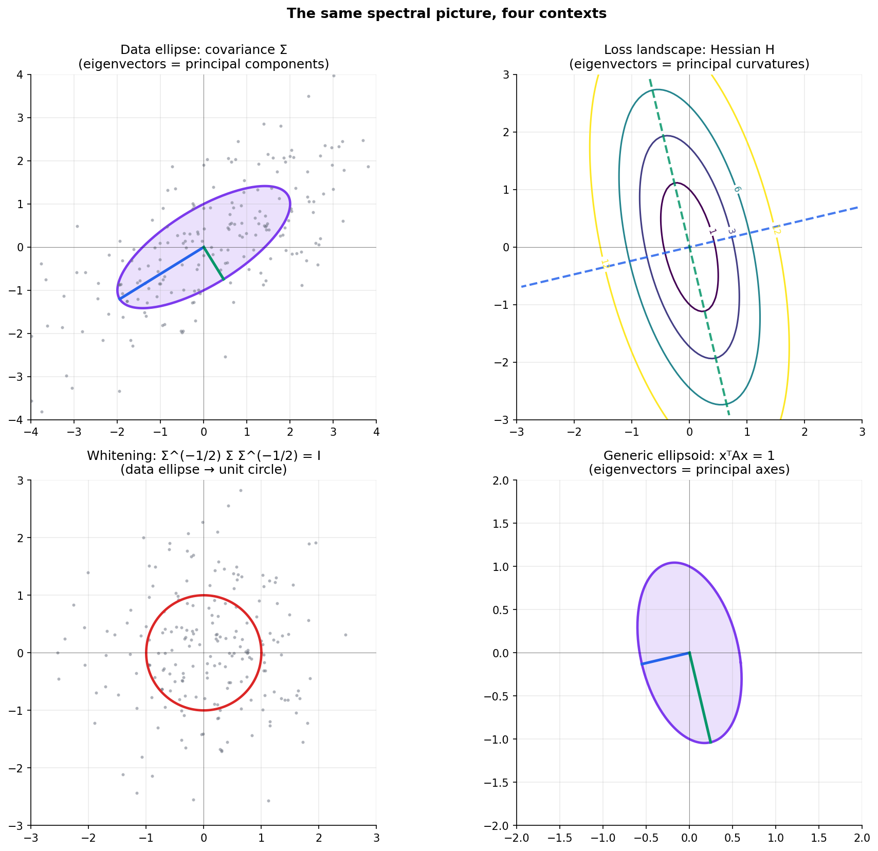
Three pictures from §§6-8 — the spectral theorem’s ellipsoid (Definition 11), the quadratic form’s level sets (Theorem 7), and the Rayleigh quotient’s extrema on the unit sphere (Theorem 9) — are the same geometric object read three ways. This short consolidating section names the unification and applies it to three apparently unrelated ML contexts that all reduce to the same spectral picture.
📐 Definition 13 (Principal Axes)
Let be symmetric positive-definite with spectral decomposition . The principal axes of are the eigenvectors . The principal-axis lengths of the unit ellipsoid are the semi-axes, equal to along .
The interpretation: a positive-definite symmetric matrix is “a uniform stretching along an orthogonal set of axes.” The axes are the eigenvectors; the stretch factors are the eigenvalues. This is the picture every covariance ellipse, every quadratic loss landscape, and every Mahalanobis ball is invoking.
🔷 Proposition 4 (Whitening Transformation)
Let be a symmetric positive-definite matrix with spectral decomposition . The whitening transformation
satisfies . Equivalently, if is a random vector with covariance , then has covariance .
Proof.
is symmetric: . So , and the conjugation simplifies:
Using (orthogonality of ) at each step: .
📝 Example 12 (Whitening a 2D Gaussian)
Let . Eigenvalues from the characteristic polynomial : , .
Eigenvectors: (high-variance direction); (low-variance direction). The data ellipse — the locus where the multivariate-normal density takes any fixed value — is an ellipse with semi-axes and , oriented along and .
The whitening transformation stretches the data along (where variance is small) and compresses along (where variance is large), so the resulting distribution is circularly symmetric. Linear regression after whitening becomes well-conditioned; Mahalanobis distance becomes Euclidean distance in the whitened coordinates.
💡 Remark 13 (The three pictures, unified)
A positive-definite symmetric matrix is simultaneously three different objects:
(a) A quadratic form whose level sets are ellipsoids (Definition 11);
(b) A linear map whose action on the unit sphere stretches it to an ellipsoid (the spectral-theorem picture from the <SpectralDecompositionVisualizer /> above);
(c) An inner product structure that defines the Mahalanobis distance .
The eigenvalues and eigenvectors are the same in all three pictures; only the visualization differs. This is the unifying observation that makes spectral methods so reusable across ML and statistics. mahalanobis-distance →
ML aside. Adam, RMSProp, and AdaGrad are approximate whitening methods for gradient descent. Each maintains a running estimate of (the diagonal of) the loss Hessian and uses it to rescale per-coordinate step sizes — effectively applying a diagonal approximation of to the gradient at each step. Full whitening would require the full eigendecomposition of the Hessian; the diagonal approximation is what is computationally tractable. The condition number from the Hessian topic is the anisotropy of the loss ellipsoid — the ratio of longest to shortest axis. Newton’s method whitens fully (uses as preconditioner) and converges in one step on a pure quadratic.
11. Connections to Machine Learning
The spectral theorem and its corollaries are the most heavily reused piece of linear algebra in machine learning. Three applications span the full breadth of the topic, each pulling on a different part of what we built. We do not develop the algorithms here — that is the job of the formalML site — but the mathematics each technique invokes is contained in this topic.
11.1. Gradient descent and the Hessian spectrum
Near a strict local minimum of a smooth loss , the gradient flow linearizes to where and . The Hessian is symmetric (Clairaut, Topic 11) and positive-definite at a strict local minimum, so the spectral theorem applies: .
Change coordinates to — the eigenbasis. The dynamics decouple into independent scalar ODEs:
Each eigencomponent decays at rate ; the slowest mode (smallest eigenvalue) dominates the long-time behavior.
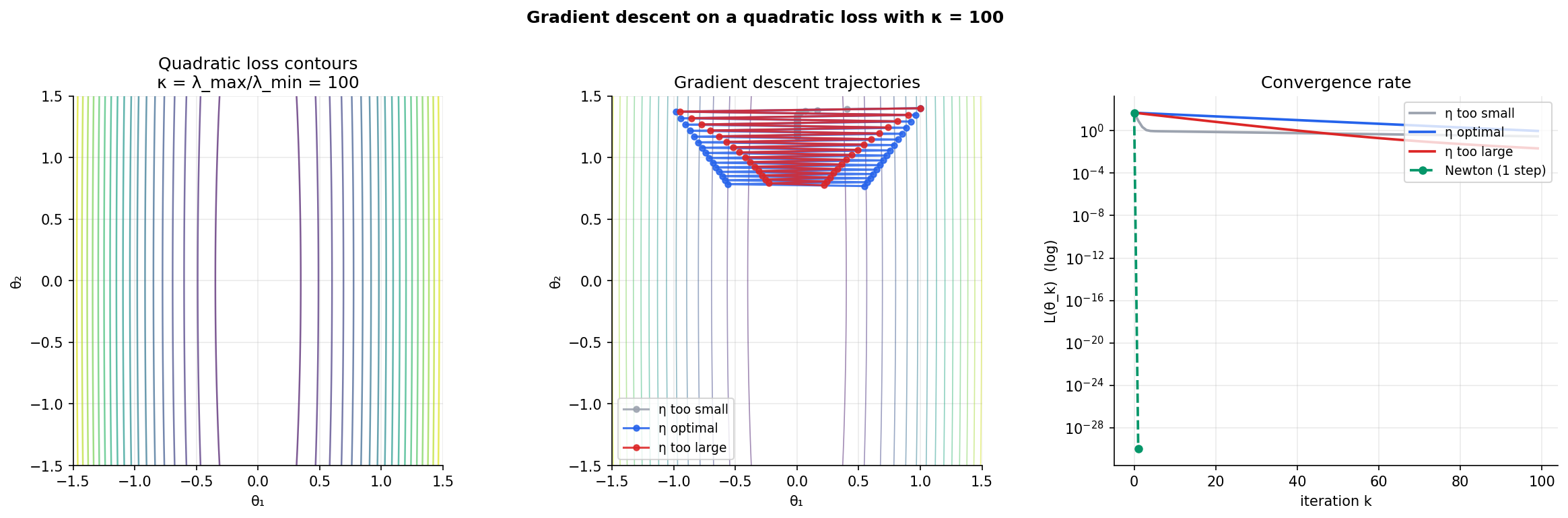
Discrete gradient descent with step size replaces with , where is the iteration count. Convergence requires for every , i.e. . The optimal step size minimizes the worst-case rate, giving convergence at rate
The condition number is the principal-axis aspect ratio of the loss ellipsoid. Ill-conditioned problems () train slowly along the small-eigenvalue direction. Newton’s method effectively rescales the dynamics to (preconditioning by ) — one step suffices for an exact quadratic loss. gradient-descent →
📝 Example 13 (Convergence rate on a quadratic loss)
Let with . Eigenvalues , , . Optimal step size .
After 100 iterations of optimal-step gradient descent, the slow direction (eigenvalue 1) has residual
Only ~87% reduction — a hundred iterations bought you about two halvings of the error. The fast direction (eigenvalue 100) has residual — about the same magnitude, but oscillating in sign because the step is “too large” for this direction. Newton’s method on the same converges in one step: .
11.2. PCA as the spectral theorem
Let be a mean-centered data matrix ( observations, features). The sample covariance is
a symmetric positive-semidefinite matrix. By the spectral theorem, with ordered non-increasingly. The columns of are the principal components ; the diagonal entries are the variances along those directions.
The first principal component is the unit vector maximizing — the direction of maximum variance. By Theorem 9 (Rayleigh quotient), the maximum is achieved at . The first components capture variance ; the explained-variance ratio is
PCA truncation to the top components gives the best rank- approximation in Frobenius norm (Eckart-Young, which we do not prove). All of this — the variance maximization, the orthogonality, the explained-variance ordering — is the spectral theorem read as a statistical procedure. PCA is the spectral decomposition of a covariance matrix. principal-components-analysis →
11.3. Spectral clustering and kernel methods
Spectral clustering. Let be a graph with weighted adjacency matrix (entries ). The graph Laplacian is
symmetric positive-semidefinite. Its smallest eigenvalue is with eigenvector (when is connected); the next smallest is the Fiedler value, and its eigenvector — the Fiedler vector — gives an approximate minimum balanced cut of by sign: vertices with positive Fiedler-vector entry form one cluster, negative the other. Spectral clustering uses the bottom nontrivial eigenvectors as features and applies -means in that feature space. spectral-clustering →
Kernel methods. A kernel is positive-semidefinite if its Gram matrix is symmetric PSD for every finite point set . Mercer’s theorem decomposes the kernel as an infinite-dimensional spectral expansion:
The finite-dimensional version is the spectral decomposition of the Gram matrix . Kernel PCA, kernel ridge regression, Gaussian-process predictive means — all of them are matrix-spectrum computations on this Gram matrix. kernel-methods →
Both constructions are the spectral theorem applied to a structured positive-semidefinite matrix. The construction is the same; only the matrix changes.
12. Where This Leads
We have built the spectral picture of symmetric matrices: orthogonal eigenvectors, real eigenvalues, the factorization , the definiteness classification, the Rayleigh quotient as a variational characterization, and Courant-Fischer as its extension to every eigenvalue. Four natural sequels extend this story in different directions, each living elsewhere in the curriculum (or on a sister site).
Singular value decomposition (SVD) extends the spectral theorem to rectangular matrices. For any real matrix — not necessarily square, not necessarily symmetric — there exist orthogonal (), (), and a diagonal (, non-negative entries called singular values) such that
The construction reduces to the spectral theorem on and (both symmetric positive-semidefinite). The geometric reading is that every linear map between inner-product spaces factors as “rotate, scale along orthogonal axes, rotate again.” SVD is the foundation of low-rank approximation (Eckart-Young), the Moore-Penrose pseudoinverse, and the bulk of modern numerical linear algebra. It is the natural next topic on this track, currently planned for a future curriculum cycle.
Principal Component Analysis (PCA) is the statistical sibling of SVD: PCA on a centered data matrix is the singular value decomposition of with the singular values squared giving the variances. We previewed PCA in §11.2; the full statistical treatment lives on formalstatistics.com, and the ML treatment on formalml.com. The mathematics is entirely contained in this topic — PCA adds no new linear algebra.
Perturbation theory of eigenvalues asks how the spectrum of relates to the spectrum of for small . Weyl’s inequality (Theorem 11) is the entry point; Bauer-Fike, Davis-Kahan, and the resolvent expansion are the next steps. The theory is essential for understanding numerical stability of eigenvalue solvers and for proving consistency results in statistical learning theory — e.g. that empirical PCA on a sample converges to population PCA as . Trefethen & Bau, Stewart-Sun, and Kato are the standard references; we do not develop perturbation theory here.
Infinite-dimensional spectral theory extends every finite-dimensional theorem in this topic to compact self-adjoint operators on a Hilbert space. The spectral theorem becomes a sum over a countable orthonormal basis of eigenvectors with eigenvalues converging to zero. The Hilbert Spaces topic states the infinite-dimensional theorem and uses it for Fourier series, Sturm-Liouville theory, and integral operators. The finite-dimensional intuition and proof developed here are exactly the right preparation for that material.
Within the Linear Algebra track, this topic completes the currently planned curriculum. Future track extensions might include SVD as a dedicated topic, quadratic forms in optimization (closing the loop with Hessian), and a numerical-linear-algebra topic covering the QR algorithm, power iteration, Lanczos, and Arnoldi. Those are deferred to a future curriculum cycle.
Connections & Further Reading
Prerequisites — topics you need first
On to formalStatistics — where this calculus powers inference
Multivariate Distributions
Spectral decomposition Σ = QΛQᵀ provides the principal-axes geometry of the multivariate normal and is the mathematical core of PCA. The contours of the density are ellipsoids whose axes are the eigenvectors of Σ and whose half-lengths are the square roots of the eigenvalues.
Principal Components Analysis
PCA on mean-centered data X solves the eigenproblem ΣQ = QΛ for Σ = XᵀX/(n−1). The principal components are the eigenvectors qᵢ ordered by descending eigenvalues λᵢ, and the variance captured by the k-th component is exactly λₖ. Every PCA derivation reduces to the spectral theorem on a real symmetric matrix.
Covariance Correlation
A covariance matrix Σ is symmetric and positive-semidefinite, so it has real non-negative eigenvalues and an orthonormal eigenbasis. The eigenvalues are the variances of the principal-component scores, and Σ is positive-definite if and only if no nontrivial linear combination of the variables has zero variance — a rank-vs-null-space statement in spectral language.
Mahalanobis Distance
The Mahalanobis distance d(x, y) = √((x − y)ᵀ Σ⁻¹ (x − y)) is the Euclidean distance in the basis where Σ becomes the identity — the whitening transformation Σ^(−1/2) is constructed by the spectral decomposition Σ = QΛQᵀ via Σ^(−1/2) = QΛ^(−1/2)Qᵀ. Mahalanobis geometry is spectral geometry in disguise.
On to formalML — where this calculus powers ML
Pca And Spectral Methods
PCA is the spectral theorem applied to a covariance matrix. The first k principal components are the top k eigenvectors of XᵀX/(n−1), and the k-dimensional projection retaining maximum variance is the projection onto their span. Spectral methods for clustering, embedding, and dimensionality reduction all instantiate the same construction on different positive-semidefinite matrices.
Gradient Descent
Gradient descent on a quadratic loss L(θ) = ½θᵀHθ decomposes along the eigenbasis of H: each eigencomponent decays at rate e^{−λᵢt} in continuous time or (1 − ηλᵢ)^k in discrete time. The condition number κ(H) = λ_max/λ_min bounds the convergence rate, and the principal-axis picture of the loss landscape — ellipsoidal level sets oriented along eigenvectors — explains why ill-conditioned problems train slowly.
Spectral Clustering
Spectral clustering uses the eigenvectors of a graph Laplacian L = D − W (or its normalized variants) to partition data points. L is symmetric positive-semidefinite, and the Fiedler vector (the eigenvector for the second-smallest eigenvalue) gives an approximate balanced cut. The construction is a direct application of the spectral theorem to a structured PSD matrix.
Kernel Methods
Mercer's theorem decomposes a positive-semidefinite kernel as K(x, y) = Σᵢ λᵢ φᵢ(x) φᵢ(y) — an eigenvalue expansion. The finite-dimensional version is the spectral decomposition of the Gram matrix Kᵢⱼ = k(xᵢ, xⱼ). Kernel PCA, kernel ridge regression, and Gaussian-process predictive means are all matrix-spectrum computations on this Gram matrix.
References
- book Axler (2024). Linear Algebra Done Right The eigenvalue-first textbook. Chapters 5 and 7 develop spectral theory before determinants — the opposite of our ordering. Read for the cleanest possible treatment of invariant subspaces, the spectral theorem for self-adjoint operators (Axler's Theorem 7.13), and the inner-product-space approach to quadratic forms.
- book Strang (2023). Introduction to Linear Algebra Chapter 6 (eigenvalues and eigenvectors) and Chapter 7 (SVD) are the closest published match to our pedagogical line for this topic. Strang's emphasis on the geometric meaning of Ax = λx — directions that don't rotate — is the framing we take.
- book Horn & Johnson (2013). Matrix Analysis The rigorous reference. Chapter 1 covers the characteristic polynomial and similarity; Chapter 2 covers unitary similarity and triangularization; Chapter 4 covers Hermitian matrices and variational characterizations (Courant-Fischer). Use for cross-checking statements; not for pedagogy.
- book Meyer (2000). Matrix Analysis and Applied Linear Algebra Chapter 7 (eigenvalues and eigenvectors) is the source for our proof of the spectral theorem via induction on dimension. The geometric pictures of quadratic forms in §7.5 are the visual templates for our principal-axes visualizations.
- book Trefethen & Bau (1997). Numerical Linear Algebra Lectures 24–30 cover eigenvalue algorithms in depth — QR iteration, Hessenberg form, divide-and-conquer. We cite this only as the right place to learn the numerical theory we explicitly do not develop. Lecture 24's discussion of why the characteristic polynomial is the wrong way to compute eigenvalues is the source for our computational-reality remark in §3.
- book Hoffman & Kunze (1971). Linear Algebra Chapter 6 (elementary canonical forms) and Chapter 7 (the rational and Jordan forms) are the standard rigorous treatment of diagonalizability and Jordan normal form. Used here as the reference for the defective-matrix detour.
- book Lax (2007). Linear Algebra and Its Applications Lax's chapters on spectral theory of self-adjoint operators and the Courant-Fischer min-max principle are the cleanest finite-dimensional treatment of the material we cover in §§7–9. Bridges naturally to the functional-analysis topics in Track 8.
- paper Pearson (1901). “On Lines and Planes of Closest Fit to Systems of Points in Space” Karl Pearson's original PCA paper. Cited as the historical origin of the principal-axes geometry of data — predates the modern statistical formulation but contains the geometric idea in its first form.