Linear Algebra
Vector spaces, linear maps, and the algebra under every calculation
Abstract. Vector spaces, linear independence, bases and dimension, linear maps and the matrices that represent them, matrix algebra defined as composition, determinants as signed-volume scaling, the rank-nullity theorem, change of basis, and inner products with orthogonality and the Gram-Schmidt process — the foundational linear-algebra substrate that every later spectral, geometric, statistical, and ML argument quietly relies on. We build the subject geometrically: a vector space is whatever adds and scales like arrows, a linear map is whatever sends lines to lines and the origin to itself, a matrix is the coordinate record of a linear map in a chosen basis, and the determinant is the signed volume scaling factor of the unit cube under the map. Composition of linear maps becomes matrix multiplication; orthogonal projection becomes least squares; the Gram-Schmidt construction becomes the QR factorization. The reader leaves this topic with the geometric reading of matrices that the rest of the curriculum — and most of machine learning — assumes silently.
1. What Linear Algebra Studies
Pick a function from the plane to itself. What is the simplest possible kind of function it could be? Not constant — that throws away too much information. Not arbitrary — most arbitrary functions are unmanageable. Somewhere in between is a class of functions that respects the geometry of the plane in a very particular way: they send straight lines to straight lines, they send parallel lines to parallel lines, and they leave the origin where it is. We call these functions linear, and linear algebra is the systematic study of what they can and cannot do.
Three pictures will set the scene. A rotation by some angle around the origin: lines through the origin rotate to other lines through the origin, parallel pairs stay parallel, and the origin stays put. A uniform stretch by some factor: every vector is rescaled, but again lines stay lines, parallels stay parallel, and the origin is fixed. A shear — imagine taking a deck of cards and pushing the top of the stack sideways while the bottom card stays still — once more, lines, parallels, and the origin all behave. These three transformations look different but share the same defining structure, and that structure is what we are going to name and study.
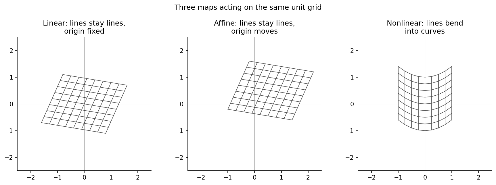
Contrast these with two non-examples. A translation — sliding every point a fixed distance in some direction — sends the origin somewhere else, so it fails the “origin stays put” condition. Translations are not linear, even though they look extremely similar to the rotations and shears we just described. We will come back to this distinction; it is the difference between a linear map and an affine map, and it is the reason every neural network layer separates a multiplication by a weight matrix from an addition of a bias vector. A quadratic warp like bends straight lines into parabolas, so it fails the “lines go to lines” condition. Quadratic warps are not linear either, and the entire reason a neural network is more expressive than a single matrix multiplication is that the nonlinearity in bends lines into curves.
ML aside. A neural network layer without the bias term and without the activation function is exactly a linear map. The bias breaks the “origin stays put” condition; the activation breaks the “lines stay lines” condition. When ML papers talk about “the linear part of a layer,” they mean the bare matrix multiplication , and that is the object linear algebra is built to study.
The plan for this topic is to take the informal picture above and make it precise. We will define what a vector and a vector space are, what it means for a function to be linear, how to record a linear map as a matrix, how matrices compose, how to read off the rank and the determinant of a matrix from its geometry, and how to choose a basis that makes a particular map look as simple as possible. By the end of the topic the reader should be able to look at a matrix and see, immediately, what it does to space.
2. Vector Spaces
Before we can talk about linear maps, we need to talk about the objects they act on. The familiar examples are arrows in the plane — directed segments with a tail at the origin and a head somewhere else — but the same algebraic structure appears in places that look nothing like arrows. The point of the vector-space abstraction is to identify exactly which properties of arrows are the ones that make the algebra work, and to declare any other set with the same properties an honorary vector space.
Start with . A vector here is a pair of real numbers, which we draw as an arrow from to . Addition is componentwise,
and geometrically the result is the head-to-tail or parallelogram sum. Scalar multiplication is also componentwise,
and geometrically the vector is stretched or shrunk (and flipped if ). These two operations satisfy eight properties — commutativity and associativity of addition, the existence of a zero vector and additive inverses, two distributive laws, and the rules for combining scalar multiplications — and any time you prove a theorem about arrows using only these eight properties, the theorem applies to any other set with the same operations. That is the move we are about to make.
📐 Definition 1 (Vector Space (over ℝ))
A real vector space is a set together with two operations,
called addition and scalar multiplication, satisfying the following eight axioms for all and :
- (Commutativity of ) .
- (Associativity of ) .
- (Zero vector) There exists with for every .
- (Additive inverses) For every there exists with .
- (Distributivity over vector addition) .
- (Distributivity over scalar addition) .
- (Compatibility of scalar multiplication) .
- (Scalar identity) .
Elements of are called vectors; real numbers in this context are called scalars.
The list looks intimidating until you notice that every one of the axioms is something you already do without thinking when you manipulate ordinary numbers — the only difference is that on the left side we have vectors instead of numbers. The axioms are not the content of the theory; they are the gatekeeper. A set with operations is a vector space exactly when all eight conditions check out, and the theorems we are about to prove apply to any such set.
📝 Example 1 (ℝⁿ)
The set of -tuples of real numbers, with componentwise addition
and componentwise scalar multiplication
is a real vector space. Verifying the eight axioms reduces to verifying them one coordinate at a time, where each verification is an instance of the familiar arithmetic of real numbers. The zero vector is , and the additive inverse of is . This is the prototype example, and most of the geometric intuition we will develop lives here.
📝 Example 2 (Continuous Functions C[a, b])
Let denote the set of continuous functions . Define addition pointwise — — and scalar multiplication pointwise — . The eight axioms hold because each one reduces to the corresponding axiom for applied at every point . Continuity is preserved because the sum of two continuous functions is continuous and a constant times a continuous function is continuous — facts established once and for all in the Sequences, Limits & Convergence topic. So is a real vector space whose vectors are functions, not arrows.
📝 Example 3 (Polynomials Pₙ)
Let denote the set of polynomials of degree at most with real coefficients,
Addition is the usual sum-of-coefficients; scalar multiplication multiplies every coefficient by the scalar. Both operations leave the degree at most , so is closed under them, and the eight axioms hold by the same coefficient-by-coefficient argument as for . The zero vector is the zero polynomial. We will see in a moment that has exactly “degrees of freedom” — the coefficients — and that this is what it means for to be “-dimensional.”
💡 Remark 1 (Why the abstraction earns its keep)
Three sets that look completely different — arrows in the plane, continuous functions on an interval, and polynomials — are all vector spaces, and we have just listed the eight properties they share. Every theorem we prove from those eight properties alone applies to all three sets at once, with no extra work. That is not a small bookkeeping convenience; it is the entire reason linear algebra is the most reusable piece of mathematics in the sciences. When you encounter a fourth or fifth example — and you will, in nearly every topic on this site — you do not have to redo the theory. You check the axioms, and then everything we are about to prove is yours.
![Three vector spaces with the same axioms: arrows in R^2, continuous functions on [0,1], polynomials in P_2](/images/topics/linear-algebra/vector-space-examples.png)
ML aside. When you concatenate a 768-dimensional BERT embedding with a 64-dimensional dense feature vector, you produce an element of the direct sum — a brand-new vector space built from two old ones. When you process a minibatch of samples, each -dimensional, you work inside . None of this is incidental: the reason these constructions compose cleanly across PyTorch and JAX is that the underlying algebra is the vector-space algebra defined above. Once you see linear algebra as the rules for combining vector spaces, every reshape and concatenate operation in ML code becomes a vector-space construction in disguise.
3. Linear Independence, Span, Basis, and Dimension
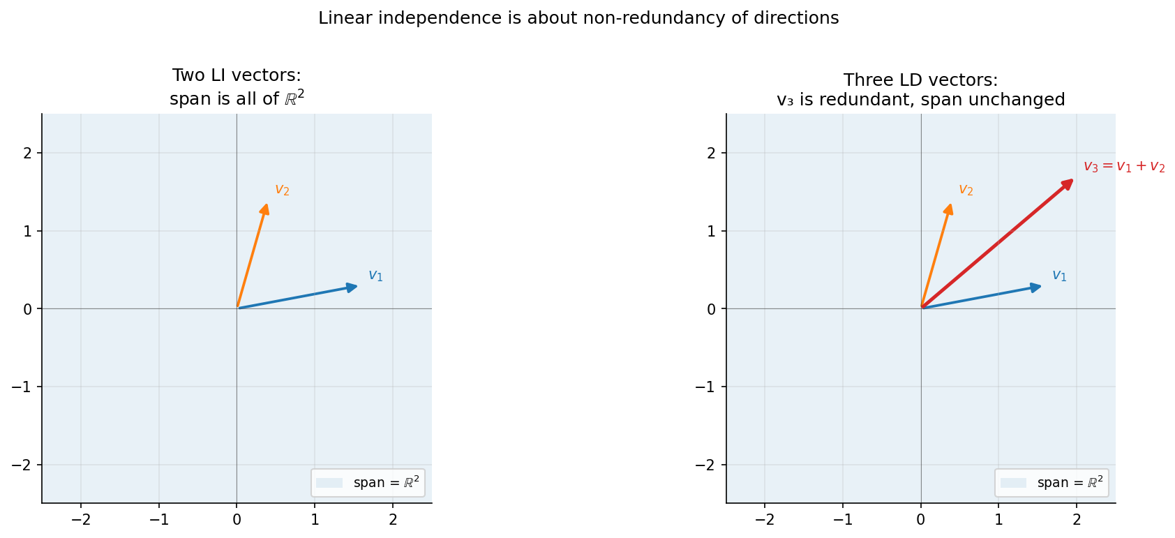
Now we put the abstraction to work. The four concepts in the title of this section — span, linear independence, basis, dimension — are the most-used vocabulary in all of linear algebra, and the right way to introduce them is geometric. Pick two arrows in that point in different directions. Can you reach any other arrow by adding scaled copies of those two? Yes: the two arrows span the plane. Pick a third arrow. Is it redundant — already reachable from the first two? Yes again: the three arrows are linearly dependent. A basis of the plane is two arrows that span without redundancy, and the number two is the dimension. Everything below is making these four sentences precise.
📐 Definition 2 (Linear Combination and Span)
Let be a vector space and let be a finite list of vectors. A linear combination of these vectors is any vector of the form
The span of , written , is the set of all linear combinations:
A span is itself a vector space — adding two linear combinations or scaling one gives another linear combination — so the span of any list of vectors is a vector space sitting inside . We call such an inner vector space a subspace. The span of one nonzero vector is a line through the origin; the span of two non-parallel vectors in is the entire plane; the span of three vectors in that don’t all lie in a common plane is the entire 3-space.
📐 Definition 3 (Linear Independence)
The vectors in a vector space are linearly independent if the only solution to the equation
is the trivial one, . They are linearly dependent if some choice of coefficients that are not all zero produces the zero vector.
Read the definition geometrically: a list of vectors is linearly dependent exactly when at least one of them can be written as a combination of the others (rearrange the equation to isolate any term with a nonzero coefficient). So “dependent” means redundant — one of the vectors carries no new directions — and “independent” means non-redundant. In , two vectors are dependent if and only if they are parallel; in , three vectors are dependent if and only if they all lie in a common plane through the origin.
📐 Definition 4 (Basis)
A basis of a vector space is a list of vectors that is
- linearly independent, and
- spans , i.e., .
A basis is the Goldilocks list: large enough to span (reach everything) and small enough to be independent (no redundancy). The standard basis of is , where is the vector with a in slot and s elsewhere; verifying that this list spans and is independent is direct. The basis of is the analog for polynomials. There are infinitely many other bases of either space — every rotation of the standard basis of produces another orthonormal basis, and any independent spanning set works — and we are about to prove that no matter which basis we pick, the number of vectors is always the same.
Before that theorem, one fact we will need repeatedly:
🔷 Proposition 1 (Unique Representation in a Basis)
Let be a basis of a vector space . Then every has a unique expression as a linear combination of the basis vectors:
The numbers are called the coordinates of with respect to the basis.
Proof.
Existence. Because the basis spans , every is some linear combination of the basis vectors.
Uniqueness. Suppose has two expressions:
Subtracting the right side from the left,
By linear independence of the basis, the only way a linear combination of can equal is if every coefficient is zero, so for each , which is . The two expressions are the same.
Coordinates are how an abstract vector space gets concrete. Once you pick a basis, every vector becomes a column of numbers — its coordinates — and you can do arithmetic with those numbers. Different bases give different coordinates for the same vector, and switching between them is what §9 of this topic (Change of Basis) will be about. For now, the bookkeeping fact is that the coordinates exist and are unique.
The headline theorem of this section is that any two bases of the same vector space have the same number of vectors. This number is well-defined and earns the name dimension.
🔷 Theorem 1 (Dimension Theorem (Steinitz Exchange))
If and are both bases of the same vector space , then .
Proof.
We prove the theorem by establishing a stronger statement called the Exchange Lemma: if spans and is linearly independent in , then . Applying this lemma twice — first to the basis (which spans) and the basis (which is independent), giving , and then with the roles reversed, giving — completes the proof.
We prove the lemma by induction on , where at step we will have replaced of the with the vectors while preserving the spanning property.
Step 1. Because spans and , we can write
At least one coefficient is nonzero — otherwise , which would contradict the linear independence of (independent sets never contain the zero vector). Reordering the if necessary, assume . Then we can solve for :
So is a linear combination of , which means still spans : anything previously reachable from the old list is still reachable from the new one.
Inductive step. Suppose after steps we have a spanning list of the form . If we are done — the inductive procedure has consumed all the , so of the original have been replaced and in particular . Otherwise, and we have at least one more to insert. Write
using the inductive spanning property. At least one of the must be nonzero, because if every were zero then would be a linear combination of , contradicting the linear independence of . Reordering the remaining if necessary, assume . Solving for as in Step 1, we conclude that is a linear combination of the new list , so the new list still spans . This completes the inductive step.
Termination. The induction can run for at most steps before we exhaust the . If at the end of the inductive procedure we still have left over — that is, if — then we would have a contradiction at step : after replacing all of the we would be trying to express as a linear combination of , which would violate linear independence. So , which is the lemma.
The Steinitz exchange argument is the workhorse of finite-dimensional linear algebra: it is also how one proves that every linearly independent set can be extended to a basis (run the exchange in reverse, adding vectors from a known basis until the set spans) and that every spanning set contains a basis (run the exchange and discard the redundant vectors). Both facts will be invoked silently in §8 when we prove the rank-nullity theorem.
📐 Definition 5 (Dimension)
The dimension of a vector space , written , is the number of vectors in any basis. By the Dimension Theorem, this number does not depend on the choice of basis, so the dimension is well-defined. A vector space is finite-dimensional if it has a basis with finitely many elements, and infinite-dimensional otherwise.
📝 Example 4 (Dimensions of ℝⁿ, Pₙ, and C[a, b])
For each of our running examples:
- , with the standard basis .
- , with basis .
- . To see this, note that the functions are linearly independent in for every (a polynomial of degree at most has at most roots, so if a nontrivial linear combination of monomials were the zero function it would have infinitely many roots — impossible). So contains as a subspace for every , and no finite basis can suffice.
The first vector-space-flavored interactive viz on this site uses these definitions directly. Drag the arrows below to manipulate a candidate basis of ; toggle vectors active and inactive; switch between presets. The readout tracks the rank of the active set (the dimension of its span), whether the set is linearly independent, and — when exactly two vectors are active — the determinant of the matrix whose columns are those vectors.
- v1 = (1.00, 0.00)
- v2 = (0.00, 1.00)
- rank = 2 (of 2 active)
- dim span = 2
- det = 1.00 (+)
- linearly independent
Drag any vector tip to change its direction and length. Toggle active to exclude a vector from the rank/determinant calculation.
A useful exercise once the viz is in hand: configure the three “dependent” vectors so that the determinant of the first two is positive, and watch the determinant flip sign when you swap them. The sign of the determinant tracks the orientation of the basis — a concept §7 will make precise.
💡 Remark 2 (Infinite-Dimensional Vector Spaces)
Most function spaces are infinite-dimensional. The space above is just one example; the space of square-integrable functions is another, and so is the sequence space of square-summable real sequences. The theorems we prove in this topic are about finite-dimensional spaces, but the language — span, basis, dimension, orthogonality — extends to infinite dimensions with appropriate care for convergence. That extension is the subject of functional analysis, the focus of Metric Spaces, Normed & Banach Spaces, and Inner Product & Hilbert Spaces elsewhere on this site. Finite-dimensional linear algebra is the warm-up; infinite-dimensional linear algebra is the real game.
ML aside. When a paper introduces a model that “projects onto a 128-dimensional latent space,” the number 128 is a dimension in exactly the sense above: it is the size of any basis of that latent space. Two architectures with the same latent dimension but different bases are representationally equivalent up to a change of coordinates — which is one reason representational similarity analysis exists, and one reason different word-embedding models with the same dimension can encode the same semantic structure in apparently unrelated coordinates. Choosing a basis for the latent space is what training the embedding layer does; the dimension is a hyperparameter you set, and the basis is a parameter the model learns.
Where this leads. We have a vocabulary now: vectors, spans, independent sets, bases, and dimensions. The natural next question — the one that animates the rest of the topic — is what functions between vector spaces look like, and the answer is the same answer that motivated this whole development: linear functions. Section 4 below introduces linear maps, and §5 explains why a matrix is exactly the right way to record one. Further out, once we have built the full apparatus, a deeper question will surface: given a linear map acting on a vector space , can we find a basis of that makes the matrix of as simple as possible? For some maps, yes: a basis of “directions the map only stretches without rotating.” Those directions have a name — eigenvectors — but they belong to the next topic on this track, and we will not introduce them here. For now, every basis is equally good.
4. Linear Maps
A function between vector spaces is a rule that takes a vector in one space and produces a vector in another. Most functions you can write down are wild — they bend lines, stretch some regions while crushing others, and have nothing in common with one another. The class of functions linear algebra studies is the narrowest possible one that respects the two operations a vector space comes with: addition and scalar multiplication. A function with this property is called a linear map (or, equivalently, a linear transformation), and the entire content of §§4-9 of this topic is what these maps can and cannot do.
The geometric picture is the one we developed in §1: a linear map sends straight lines through the origin to straight lines through the origin (possibly degenerated to a single point), parallel lines to parallel lines, and the origin to itself. Algebraically, “respects addition and scalar multiplication” turns into two equations that we elevate to definition.
📐 Definition 6 (Linear Map)
A function between real vector spaces is a linear map (or linear transformation) if it satisfies the two structure conditions
- (Additivity) for all .
- (Homogeneity) for all and all .
Equivalently — and this single equation is sometimes used as the definition — for all scalars and all vectors .
One immediate consequence of the two axioms is that every linear map sends the zero vector to the zero vector: . This is the algebraic shadow of the geometric “origin stays put” condition from §1, and it is the single property that distinguishes a linear map from an affine one (which is a linear map composed with a translation). Now four examples — the canonical zoo of linear maps on the plane — each of which the reader should be able to draw from memory by the end of this section.
📝 Example 5 (Rotation by θ in ℝ²)
For a fixed angle , define by
Linearity is direct from the formula: each output coordinate is a real-linear combination of and , so additivity and homogeneity in the input both go through. Geometrically, rotates every vector counter-clockwise by radians around the origin. The image of the standard basis is and — a fact that will determine the matrix of in §5.
📝 Example 6 (Orthogonal Projection onto a Line)
Let be a unit vector. The orthogonal projection onto the line spanned by is the map defined by
where is the standard dot product. Linearity follows because the dot product is linear in its first slot: . Geometrically, sends every vector to its shadow on the line through the origin in the direction of . The image of is exactly that line; its kernel is the hyperplane perpendicular to — every vector orthogonal to has and so projects to the origin.
📝 Example 7 (Uniform Scaling by λ)
For a fixed , define by
Linearity is immediate: . The geometry depends on the sign of : for the map stretches every vector outward (or shrinks toward the origin if ); for it stretches and flips through the origin; for it crushes the whole space to a single point.
📝 Example 8 (Horizontal Shear)
For a fixed , define by
Each output coordinate is a linear combination of the inputs, so is linear. Geometrically, every point’s -coordinate is preserved but its -coordinate is bumped sideways by times . The result is that horizontal lines slide rigidly, with the slide distance proportional to height: the -axis stays put (everything on it has ), and lines parallel to the -axis stay parallel — they just shift sideways. This is the “deck of cards” picture from §1 made precise.
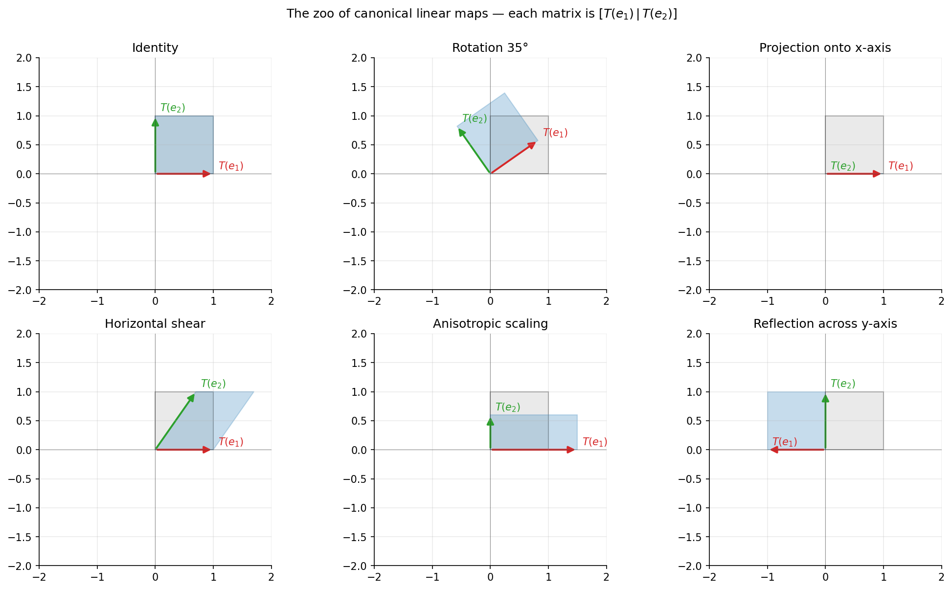
The four examples share a structural pattern. Each is determined by where it sends the two basis vectors of — once you know and , linearity tells you for every input vector. The next viz makes this pattern visceral: drag the two image vectors and watch the entire grid follow. A side panel keeps track of the matrix whose columns are exactly those image vectors — but we have not built the language of matrices yet; that’s what §5 is for. For now, the viz is a preview.
The map that does nothing. Every vector is its own image.
Column 1 is the coordinate vector of T(e₁); column 2 is the coordinate vector of T(e₂). The matching colored border ties each column to its arrow in the canvas.
|det| is the area of the parallelogram. Sign tracks orientation: positive when T preserves it, negative when reflected, zero when collapsed to a line.
Drag T(e₁) or T(e₂) to change the linear map; the matrix and the parallelogram update live. Selecting a preset animates the arrows to the target positions.
The “preset” dropdown switches between the eight canonical maps — identity, two rotations, two projections, a shear, a uniform scaling, and a reflection. The matrix readout on the right shows what those image vectors look like as a 2×2 array. The determinant indicator beneath the matrix tracks the signed area of the parallelogram in the canvas: positive for orientation-preserving maps, negative for orientation-reversing ones, zero whenever the map collapses the plane to a line.
Two subspaces are naturally associated with every linear map: the inputs that get sent to zero, and the outputs that actually get hit. They have names.
📐 Definition 7 (Kernel and Image)
Let be a linear map between vector spaces.
- The kernel (or nullspace) of is the subset of that sends to the zero vector of :
- The image (or range) of is the subset of consisting of all vectors that are hit by something in :
For the four canonical examples: rotation has trivial kernel and image all of (it loses no information and reaches every output). Projection onto the line through has kernel equal to the perpendicular line and image equal to the line through . Uniform scaling has trivial kernel and image all of when ; when the kernel is the whole space and the image is just the origin. Horizontal shear has trivial kernel and image all of . These observations are not coincidences — they are diagnostics, and §8 (Rank-Nullity) will package them into a single counting theorem.
🔷 Proposition 2 (Kernel and Image Are Subspaces)
For any linear map , the kernel is a subspace of and the image is a subspace of .
Proof.
We verify the two closure conditions and the zero-vector condition for each.
The kernel. Let and . Then by linearity,
so , and
so . The zero vector is in because (a consequence of homogeneity at ).
The image. Let , so and for some , and let . Then
and
The zero vector is in because .
💡 Remark 3 (Kernel and Nullspace Mean the Same Thing)
Pure-mathematics texts say kernel; applied texts say nullspace. They denote the same set. We use both interchangeably, preferring kernel in abstract discussion of linear maps and nullspace when discussing computations with matrices, where “the nullspace of ” is the standard phrase. Likewise, range and image are synonyms, with the same prose-vs-computation split.
The next remark is the single most consequential observation of the section, and it is the entire reason matrices exist.
💡 Remark 4 (A Linear Map is Determined by Its Action on a Basis)
Let be a finite-dimensional vector space with basis , let be any vector space, and let be any vectors in (chosen however you like — they need not be a basis, they need not be distinct, they need not even be nonzero). Then there is exactly one linear map satisfying for every .
Why. Existence: every has a unique expansion by Proposition 1, and we are forced to define in order for linearity to hold. Verifying that this definition is indeed linear is a mechanical check: linearity in the coefficient list follows from linearity in the coordinates. Uniqueness: if two linear maps and both send to for every , then they agree on the basis, and by linearity they agree on every linear combination of basis vectors, i.e. on every vector in .
This single fact is the reason a linear map is recorded by a finite block of numbers — once you have specified where each of the basis vectors goes, the whole map is determined. The next section turns that block of numbers into a matrix.
ML aside. A linear regression model is a linear map . The kernel is the hyperplane — exactly the set of input vectors at which the model predicts zero, which is the decision boundary at output 0 in machine-learning vocabulary. The image is either all of (when ) or the single point (when and the model is degenerate). The kernel/image dichotomy is exactly the geometric reading of “which inputs the model ignores” and “which outputs the model can produce” — vocabulary every regression diagnostic uses without naming.
Where this leads. We have a definition of linear map and a zoo of examples. The next two sections turn the verbal definition into a computational object — a matrix — and then describe how matrices compose. Further on, once we have all of this in hand, we will ask: among the bases we could choose for , is there one that makes the matrix of as simple as possible? For uniform scaling, every basis is equally good — every direction is just scaled. For rotation by an angle other than or , no real basis makes the matrix diagonal — every direction genuinely turns. For projection, a basis aligned with the projection line and its perpendicular reduces the matrix to a diagonal of zeros and ones. The general theory of “which maps admit a diagonalizing basis, and what does the basis look like” is the content of Eigenvalues & Eigenvectors — the next topic.
5. Matrices as Representations of Linear Maps
A matrix is, in the most reductive description, a rectangular block of numbers. That description is true and unhelpful — it is also the description that drives most students to memorize the row-by-column multiplication rule without understanding where it came from. We will give a different description: a matrix is the coordinate-dependent record of a linear map, and the row-by-column rule is the consequence, not the postulate. Once that ordering is in place, every matrix manipulation downstream becomes a geometric statement.
Here is the setup. Pick a basis of the domain and a basis of the codomain . By Remark 4, the linear map is determined by the image vectors . Each lives in and so has a unique expansion in the basis :
The scalars assemble into an rectangular array. That array is the matrix of , and reading it correctly is the entire point of this section.
📐 Definition 8 (Matrix of a Linear Map)
Let be a linear map between finite-dimensional vector spaces, let be a basis of , and let be a basis of . Write the image of each in the basis as
The matrix of relative to and , written , is the array . Equivalently — and this is the picture worth carrying around — the -th column of is the coordinate vector of in the basis .
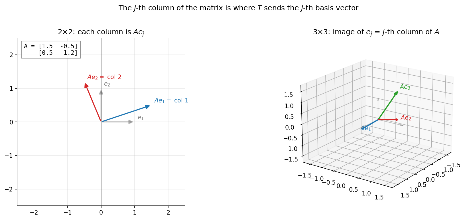
Reread that last sentence; it is what the rest of this topic rests on. The -th column is the answer to the question “where does send the -th input basis vector?” The viz above made this visible: when you drag , only the first column of the matrix changes; when you drag , only the second column changes. Read this way, the matrix is the recipe for what does to each input basis vector, written out in coordinates.
That recipe extends to every input vector — not just basis vectors — through a single computation that we now also name.
📐 Definition 9 (Matrix-Vector Product)
Let be an matrix with columns , and let be a column vector. The matrix-vector product is the vector in given by
That is, is the linear combination of the columns of with weights coming from .
The conventional formula for the matrix-vector product, , is the entry-by-entry rewrite of the columns-as-vectors formula above; they describe the same operation. Most computational packages implement the entry-by-entry form (it is friendlier to the cache), but the columns-as-vectors form is the one that makes the geometry visible. With this definition in hand, the matrix of does what its name promises.
🔷 Theorem 2 (Matrix-Vector Product Computes the Linear Map)
With notation as in Definitions 8 and 9: if has coordinate vector in the basis , then the coordinate vector of in the basis is the matrix-vector product , where .
Proof.
Start with the expansion of in and apply , using linearity at each step:
By Definition 8, . Substituting and swapping the order of the (finite) sums,
The expression in parentheses is exactly the -th entry of the matrix-vector product , so the -th coordinate of in is . That is the claim.
The theorem turns the abstract definition of a linear map into a concrete computation. To apply to a vector , write in coordinates in the input basis, look up the matrix , multiply, and read off the answer in the output basis. Every linear-algebra library on every platform does exactly this. Two examples make the matrix-of-a-map idea concrete.
📝 Example 9 (Standard Matrix of a Rotation in ℝ²)
The rotation from Example 5 sends the standard basis to
By Definition 8, those two image vectors are the columns of in the standard basis:
Applying Theorem 2 with recovers the formula from Example 5 — exactly as expected. The viz’s “Rotation by 30°” and “Rotation by 90°” presets are this matrix at and respectively.
📝 Example 10 (Matrix of Projection onto the x-axis)
Let be the map . Then and , so
The second column is all zeros, which is exactly the statement that — read columnwise. Whenever you spot a zero column in a matrix, you have spotted a basis vector in the kernel. This is the first of many “structural facts of the matrix that you read off geometrically without computing anything” the topic will accumulate.
💡 Remark 5 (Why the Columns Are the Images of Basis Vectors)
The single most important fact of linear-algebra pedagogy — the one most often skipped over in undergraduate courses and the one that makes the viz above the centerpiece of this section — is that the -th column of a matrix is the place the -th basis vector lands. Once that is internalized, almost every matrix manipulation becomes a geometric statement:
- A column of zeros means the corresponding basis vector is in the kernel.
- Two equal columns mean the matrix sends two basis vectors to the same image, so the kernel contains the difference.
- A square matrix has linearly independent columns if and only if no two input basis vectors collide and none collapses to zero, which is exactly the condition that is invertible.
- The image of a matrix is the span of its columns — period. The “column space” of a matrix and the image of the underlying linear map are the same set.
Every one of those statements is just Definition 8 plus a moment’s thought about what linear-combination means. The standard order of pedagogy reverses this — first the row-by-column rule, then the geometric consequences — but reversing the ordering loses the reason the row-by-column rule looks the way it does. We will return to this picture repeatedly; treat it as the topic’s central image.
ML aside. A fully-connected (dense) layer without bias and without nonlinearity is the map , where is a learned weight matrix. The -th column of is, by exactly Definition 8, what this layer does to the -th input neuron — its “response pattern” when only neuron is active. One popular interpretability technique is to literally render those columns as images (for image inputs) or words (for embedding inputs) and see what the layer has learned to “look for.” When you read a paper that visualizes the “feature detectors” of a neural network’s first layer, you are looking at columns of rendered as pictures — Definition 8 doing interpretability work.
6. Matrix Algebra
We now have one matrix per linear map. The next question is what happens when we combine linear maps. The two combinations that matter — composition (do one map, then another) and scaling/addition of maps — give matrix operations: matrix multiplication, scalar multiplication of matrices, and matrix addition. The standard undergraduate course postulates the rules for these operations (especially the row-by-column rule for multiplication) and asks the student to verify that they have nice properties. We do the reverse. Composition of linear maps is the more fundamental operation, and we derive the row-by-column rule as the formula that records it. The pedagogical commitment of this section is that matrix multiplication is defined to be composition; the row-times-column arithmetic is the consequence.
This ordering matters far beyond this section. The chain rule for Jacobians, the spectral theorem, the diagonalization of a covariance matrix, the composition of layers in a neural network — every downstream concept becomes a matrix-multiplication statement, and every one of them is easier to see if you read matrix multiplication as composition rather than as a memorized formula.
📐 Definition 10 (Composition of Linear Maps)
Let and be linear maps. Their composition is the function
The composition of two linear maps is itself linear: , applying the linearity axioms of once and of once.
So the composition is itself a linear map, and therefore it has a matrix. The question of this section is: what is that matrix? We answer it by chasing where each basis vector of ends up under the composition, expressing the result in coordinates, and reading off the rule.
📐 Definition 11 (Matrix Product)
Let be an matrix and be an matrix. The matrix product is the matrix whose entry is
That is the row-by-column rule, written out. We are naming it for now; we have not yet motivated it. The next theorem motivates it — by showing that is the matrix that records the composition whenever is the matrix of and is the matrix of .
🔷 Theorem 3 (Matrix Product Computes Composition)
Let and be linear maps between finite-dimensional vector spaces. Fix bases of , of , and of . Let
be the matrices of and in those bases. Then the matrix of the composition in the bases and is the matrix product
Proof.
We chase where each basis vector of ends up under the composition and read off the result columnwise, since by Definition 8 the -th column of is the coordinate vector of in the basis .
Write the bases as , , , with an matrix and an matrix.
Step 1: apply to . By Definition 8 applied to ,
Step 2: apply to the result. Using linearity of to pull the sum out, then Definition 8 applied to to expand each ,
Step 3: swap the order of summation and read off the coordinates. The two sums are finite, so we may interchange them:
The parenthesized quantity is the -th coordinate of in the basis . By Definition 8, that quantity is the entry of the matrix .
Step 4: recognize the row-by-column rule. Compare to the right-hand side of Definition 11:
The two expressions are literally identical. So the entry of equals the entry of the matrix product , for every and every . The two matrices are equal entrywise, hence equal as matrices.
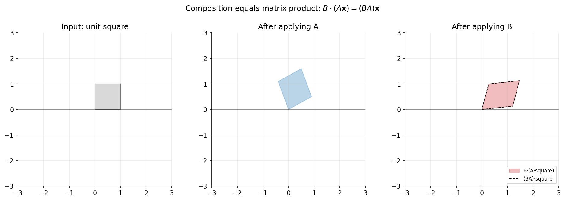
This is the structural fact the entire row-by-column rule descends from. The rule is not arbitrary; it is the unique formula that records the composition of two linear maps in coordinates. Three immediate consequences worth noticing:
- The number of columns of must equal the number of rows of , because the basis of has to match between “where sends things” and “where takes them from.”
- The result has the row count of and the column count of — the rows of the outer map and the columns of the inner one.
- The order (not ) is the order that records — outermost map on the left. We apply first to a vector and then , but we write the matrix product with ‘s matrix first. This is the conventional inconsistency that occasionally trips up newcomers; the proof above is what fixes the order.
The remaining operations on matrices — transpose, scalar addition, inverse — flow from the same recipe. Each is the matrix-side mirror of a natural operation on linear maps.
📐 Definition 12 (Transpose)
The transpose of an matrix is the matrix whose entries are . Equivalently, the rows of are the columns of and vice versa.
Geometrically, the transpose is the matrix of the adjoint of the linear map with respect to the standard inner product — a fact we will only state here and develop fully in §10 (and again in the Hilbert Spaces topic on the functional-analysis track). For now, the operation is just an entry-swapping rule.
📐 Definition 13 (Identity Matrix and Invertibility)
The identity matrix of size , written , is the matrix whose entries are
It is the matrix of the identity linear map (sending every to itself) in any basis.
A square matrix of size is invertible if there exists a matrix of the same size satisfying
When such an exists it is unique, and it is called the inverse of .
By Theorem 3 (and the fact that the identity map has the identity matrix in any basis), is invertible if and only if the linear map it represents has a two-sided inverse — i.e., is a bijection. Section 8 will collect this with several other equivalent characterizations of invertibility into a single corollary; for now, just note that “invertible” is a property of the underlying linear map, not of the bookkeeping that records it.
🔷 Proposition 3 (Properties of Matrix Algebra)
For matrices of compatible sizes and scalars :
- (Associativity of multiplication) .
- (Distributivity) and .
- (Transpose of a product) . Note the order reversal.
- (Non-commutativity) In general, . Matrix multiplication is not a commutative operation.
Properties (1) and (2) are immediate from Theorem 3 once you recognize the matrix-side claims as the matrix-side mirrors of well-known statements about functions: function composition is associative (), and linearity gives the two distributive laws automatically. Property (3) — the order reversal under transpose — is a one-line entry-wise computation that we’ll work in §10 once inner products give the operation a geometric meaning. Property (4) is the one worth dwelling on: it is the matrix-side reflection of the fact that function composition is not commutative. “First rotate, then shear” and “first shear, then rotate” are genuinely different procedures that produce different output vectors from the same input.
📝 Example 11 (Non-commutativity Made Geometric)
Let be the matrix of rotation by and be the matrix of the horizontal shear with :
Compute both orderings directly:
The two products are different. Geometrically, applies the shear first and then the rotation: the standard square is sheared into a parallelogram and then that parallelogram is rotated . rotates first and then shears: the square turns into a different square, which is then sheared into a different parallelogram. Both endings have the same area (because — the product of determinants), but they sit in different places and have different shapes. Non-commutativity is a structural feature, not a quirk of the formula.
💡 Remark 6 (Geometric Meaning of the Inverse)
A square matrix of size is invertible if and only if the linear map it represents is a bijection — every output is hit by exactly one input. That single geometric condition is equivalent to all of the following, which §8 will collect into a single corollary by the rank-nullity theorem:
- ‘s columns are linearly independent (no redundancy among the basis-vector images).
- ’s rank is (the image fills ).
- (no inputs other than zero are sent to zero).
- (the parallelepiped spanned by the columns has nonzero volume — §7).
- The system has a unique solution for every .
The remarkable fact is that all of these conditions are equivalent — they are the same statement read different ways through the rank-nullity theorem. We will prove their equivalence in §8. Until then, treat them as a single rich notion of “the matrix represents an honest one-to-one onto linear map,” and use whichever of the five characterizations is convenient at the moment.
ML aside. Stacking layers in a neural network — without the biases and the nonlinearities — computes , a single matrix product by Theorem 3. The reason a deep linear network “collapses” to a single effective matrix, and therefore has the same expressive power as a one-layer linear model, is exactly the composition rule of this section: composing linear maps gives a linear map, and the matrix of the composition is the product of the matrices. The reason deep networks are interesting at all is the nonlinearity between layers: applying after each linear step breaks the composition collapse, because composing a linear map with a nonlinear function is no longer linear and the matrix-product shortcut no longer applies. Every “depth” argument in deep learning theory works through this distinction.
7. Determinants — Signed Volume
Every square matrix has a single number attached to it called its determinant. In the standard pedagogy that number arrives as a formula — for a matrix, ; for a matrix, an alternating sum that no one remembers; for an matrix, an unwieldy sum over permutations — and students are asked to memorize the formula and verify a list of properties. That formula is correct, but it hides the meaning of the number it computes. We approach the determinant differently: we define it by the three properties it must have, prove those properties force a unique function, and then derive the formula as a consequence. The number that emerges has a clean geometric meaning — it is the signed scaling factor of the unit cube under the linear map represented by the matrix — and once that meaning is in hand, every property of the determinant becomes obvious.
The three properties are: multilinearity (linear in each column when the others are held fixed), alternating (swapping two columns negates the value), and a normalization fixing the value on the identity matrix. Each of those is a geometric statement about signed volume in disguise.
📐 Definition 14 (Determinant (Axiomatic))
The determinant of an matrix with columns is the unique function satisfying:
- (Multilinear in each column) For any column index , any scalars , and any vectors ,
The same property holds in every column, with all other columns held fixed.
-
(Alternating) Swapping two columns negates the determinant. Equivalently, if two columns are equal, the determinant is zero.
-
(Normalization) , where is the identity matrix.
Calling this a definition is doing a lot of work — we are asserting that exactly one function satisfies all three properties, and we have not yet proved that. The next theorem closes that gap.
🔷 Theorem 4 (Existence and Uniqueness of the Determinant)
There exists a unique function satisfying axioms (D1), (D2), (D3) of Definition 14. Explicitly,
where denotes the symmetric group of all permutations of and is the sign of the permutation .
Proof.
Uniqueness. Suppose satisfies (D1), (D2), (D3). Write each column of as a linear combination of the standard basis vectors,
Apply multilinearity (D1) to expand over each column index:
By the alternating property (D2), vanishes whenever any two of the indices coincide — repeated columns force the value to zero. The only surviving terms in the sum are those where is a permutation of , i.e., for some .
For such a permutation, is obtained from by some number of column swaps that bring the permuted basis back into standard order. Each swap negates the value by (D2), and the parity of the required number of swaps is exactly . Therefore
Substituting back,
which is the claimed formula. So any function satisfying (D1), (D2), (D3) must agree with that formula — uniqueness.
Existence. Take the formula in the theorem statement as a definition of , and verify directly that it satisfies (D1), (D2), (D3). Multilinearity (D1) follows because each term is linear in each column. The alternating property (D2) holds because swapping two columns of corresponds to composing with a transposition, which flips in every term; the sum therefore negates. Normalization (D3) holds because for the only nonzero product is the one with the identity permutation, contributing . So the formula defines a function satisfying all three axioms, and by uniqueness it is the only such function.
The explicit formula has terms — manageable for (two terms: ) and arguably (six terms), useless past . We will compute determinants in practice not by the permutation sum but by row reduction, which is . The permutation formula is the certificate that the function is well-defined; the computation is something else entirely. The axioms are also what give the determinant its meaning.
🔷 Theorem 5 (Geometric Meaning of the Determinant)
For any matrix with columns :
- The absolute value equals the -dimensional volume of the parallelepiped spanned by the columns of — equivalently, the volume of the image of the unit -cube under the linear map .
- The sign tracks orientation: positive if preserves the orientation of the standard basis, negative if it reverses it, zero if the columns are linearly dependent (in which case the image collapses to lower-dimensional volume zero).
Proof.
Two dimensions. The parallelogram with sides and has signed area
which can be derived by computing the area as base × height and tracking orientation: the base has length , the height is the perpendicular drop from the tip of onto the line spanned by , and the sign of the cross product records whether the columns turn counter-clockwise (positive) or clockwise (negative) as you walk . The right-hand side is exactly the determinant from the permutation formula, so the case is verified directly.
General . The signed-volume function of the parallelepiped spanned by vectors in satisfies exactly the three axioms (D1), (D2), (D3):
- Multilinearity in each column. Holding fixed, the signed volume is linear in — geometrically, doubling one side doubles the volume, and the volume of a parallelepiped with one side decomposed as splits cleanly along that decomposition (a fact derivable by Cavalieri’s principle in the appropriate dimension, made precise in Multiple Integrals & Fubini’s Theorem).
- Alternating. Swapping two columns flips the orientation of the spanning vectors and negates the signed volume; repeated columns force the parallelepiped to be degenerate and the volume to be zero.
- Normalization. The unit -cube has volume , so .
By the uniqueness clause of Theorem 4, the function and the function are equal on every input. Therefore is the signed volume of the parallelepiped spanned by the columns of for every .
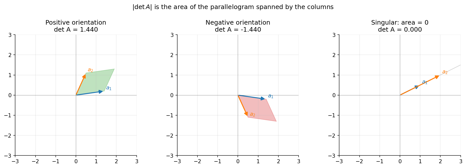
The determinant is therefore not really about the formula — it is about the volume. The viz below makes this concrete in two dimensions: drag the two column vectors and watch the parallelogram fill with green when the orientation is positive, red when negative, and grey when the columns are parallel and the parallelogram collapses to a line.
The unit square remains the unit square. Area 1.
- a₁ = (1.00, 0.00)
- a₂ = (0.00, 1.00)
- det A = 1.00
- |det A| = 1.00 (area of the parallelogram)
- positive (orientation-preserving)
Drag a₁ or a₂ to change the columns. The parallelogram colors green when det A > 0 (orientation-preserving), red when det A < 0 (orientation-reversing), grey when det A = 0 (the columns are parallel).
A useful exercise once the viz is in hand: configure the columns so the determinant equals , then add the second column to the first (the matrix becomes column-row equivalent: replace with ). Observe that the parallelogram changes shape — but its signed area does not change. That observation is the geometric content of property (c) below.
With the geometric meaning in place, the standard computational properties of the determinant become easy reading.
🔷 Theorem 6 (Computational Properties of the Determinant)
For square matrices and of the same size and a scalar :
- (Multiplicativity) .
- (Transpose) .
- (Column-addition invariance) Adding a scalar multiple of one column to another leaves the determinant unchanged.
- (Column scaling) Multiplying one column by multiplies the determinant by . Multiplying every column by multiplies the determinant by .
- (Invertibility) if and only if is invertible.
Proof.
We prove (a) — multiplicativity — in full and sketch the rest, all of which follow from Definition 14 plus simple inspection of the formula.
Multiplicativity. Suppose first that . Define the function by
We claim satisfies axioms (D1), (D2), (D3) of Definition 14 as a function of (with held fixed). The columns of are , where is the -th column of . As a function of :
- Multilinear in each column of . Each column of is a linear combination (with weights from ) of the columns of , so is multilinear in each column of by multilinearity of applied to each column of .
- Alternating in the columns of . Swapping two columns of swaps the corresponding columns of , which negates by (D2) for .
- Normalization. When , , so .
By the uniqueness clause of Theorem 4, . Rearranging gives , as claimed.
When : by (e) (proved next), is singular, so its columns are linearly dependent and has a nonzero solution. Then , so is also singular and . The identity holds either way.
Transpose. From the permutation formula,
Reindexing the product by (so ) and noting recovers exactly the formula for .
Column-addition invariance. If we replace with (for ), by multilinearity (D1) the determinant becomes . The second term has two equal columns (both equal to , one in slot and one in slot ), so it vanishes by (D2). The result equals .
Column scaling. Direct from multilinearity (D1): scaling one column by scales the determinant by . Scaling every column by does so times, giving .
Invertibility. If is invertible, then , so by (a), , which forces . Conversely, if is singular, its columns are linearly dependent, so one column is a linear combination of the others, and by (D1) the determinant decomposes into terms each of which has a repeated column — all zero by (D2). Therefore .
The computational fact behind row reduction follows immediately.
📝 Example 12 (Determinants of 2×2 and 3×3 Matrices)
For a matrix, the permutation formula gives
For a matrix, the cofactor expansion along the first row gives
These are the only sizes for which the closed-form formula is reasonable to apply by hand. For the formula has terms; for , terms; for , more than three million. Row reduction is the algorithm you actually use.
💡 Remark 7 (Why Cofactor Expansion is a Coda)
Cofactor expansion — the formula every undergraduate memorizes for matrices, generalizing in the obvious way to larger sizes — is useful for and essentially nothing else. The cost of cofactor expansion at size is , which is unusable past . The cost of row reduction is , which scales to matrices of millions of rows in scientific computing. In practice, every modern linear-algebra library computes determinants by some variant of LU decomposition — row reduction with bookkeeping — and never by cofactor expansion.
We mention cofactor expansion in this topic for two reasons. First, it generalizes the explicit formula for matrices to in a way that students can verify on paper. Second, it underlies one elegant theorem (the adjugate formula for the inverse, ), which we will not develop here but which appears in proofs of formulas relating determinants to inverses. Both are computational dead ends past small sizes.
Algorithm: determinant by row reduction. Given a square matrix of size , apply Gaussian elimination with partial pivoting to reduce to upper triangular form, tracking row swaps and row scalings as you go. After reduction,
The cost is . This is the algorithm the determinant function in linearAlgebra.ts implements (see the shared module created in slice 1); the topic’s notebook verifies its outputs against NumPy’s reference implementation across random matrices.
ML aside. When training a normalizing flow — a deep-learning architecture that learns a sequence of invertible transformations mapping a complex data distribution to a simple base distribution (typically a standard Gaussian) — the loss function involves a log-determinant of the Jacobian of each layer. The reason traces exactly to Theorem 5: a probability density transforms under a change of variables by the inverse of the Jacobian’s volume scaling, and that scaling is . Computing at scale for layers of millions of dimensions is what makes normalizing-flow architectures interesting: practitioners design layers whose Jacobians are triangular (so the determinant is the product of diagonal entries — back to a one-liner via row reduction), or block-triangular, or otherwise structured so the log-determinant is cheap. The trade-off between expressiveness and Jacobian-cheapness is the central design axis of the field. Every architecture in that literature — RealNVP, Glow, Neural ODEs, FFJORD — is a different answer to “how do we get expressive layers without paying for the determinant at every step?“
8. Rank, Nullspace, and the Rank-Nullity Theorem
Every linear map carries a pair of subspaces alongside it: the kernel (the inputs that get crushed to zero — Definition 7) and the image (the outputs that actually get reached — also Definition 7). Their dimensions are the nullity and the rank of the map respectively, and they are connected by a single counting equation — the rank-nullity theorem — that is the most useful dimension fact in finite-dimensional linear algebra. The theorem says: every dimension of the input space gets accounted for, either by getting absorbed into the kernel or by surviving as an independent direction in the image. Nothing is lost in translation; every input direction has a place to go.
The version stated in textbooks is one equation. The reason it deserves so much attention is that it unifies several apparently different statements about square matrices — invertibility, full-rank columns, full-rank rows, nontrivial null space, nonzero determinant — into a single corollary in which they are all equivalent. After we prove the main theorem, we collect those statements as Corollary 1; the equivalence is, in a real sense, the headline result of the section.
📐 Definition 15 (Rank and Nullity)
Let be a linear map between finite-dimensional vector spaces, and let be its matrix in any chosen bases.
- The rank of (or of ) is , the dimension of the image.
- The nullity of (or of ) is , the dimension of the kernel.
For an matrix , equals the dimension of its column space (equivalently, of its row space — a fact we establish in Remark 8 below), and is the dimension of its nullspace .
The rank and nullity are independent of which bases were used to write down the matrix — they are properties of the underlying linear map, not of the bookkeeping. Both are non-negative integers, both can be computed by row reduction (the rank is the number of pivots; the nullity is the number of free columns), and both are constrained by the input dimension via the theorem below.
🔷 Theorem 7 (Rank-Nullity)
For any linear map between finite-dimensional vector spaces with ,
Equivalently, for any matrix , (the number of columns).
Proof.
Let and , so . Pick a basis of (the case means we pick the empty basis). Because every linearly independent subset of extends to a basis (a consequence of the Steinitz Exchange argument from §3, applied in reverse), we can extend to a basis
of all of . The claim is that the images form a basis of . If this is true, the dimension of the image is , which gives , the theorem.
Spanning. Let , so for some . Expand in the basis ,
Applying and using linearity,
since each . So is a linear combination of , which means these vectors span .
Linear independence. Suppose
By linearity, , so the vector lies in . But has basis , so we can write
for some scalars . Rearranging,
But the combined set is a basis of , hence linearly independent. So every coefficient in the equation must be zero: for all and for all . In particular, every , which is what linear independence of requires.
Both halves of the claim are verified, so is a basis of , hence , and .
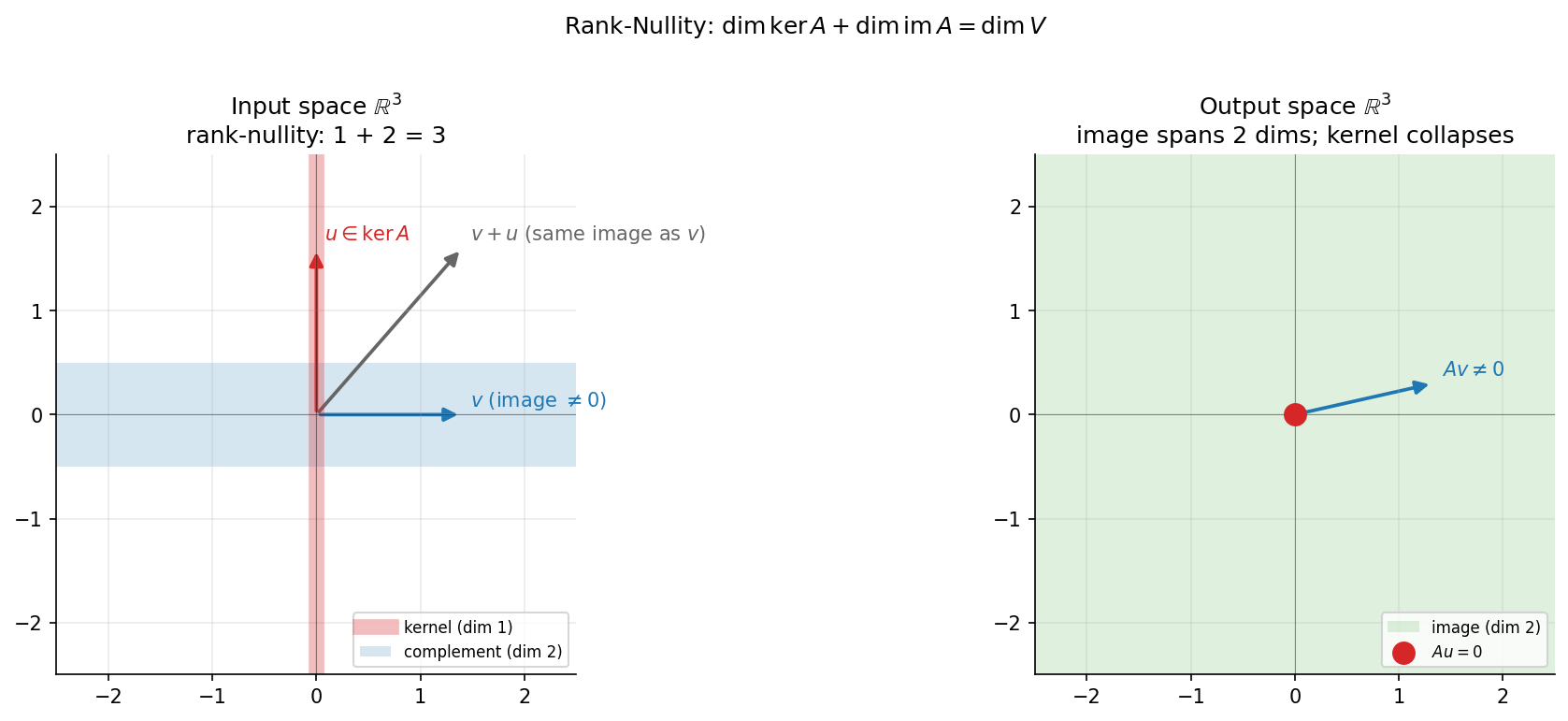
The proof has an underrated feature: it is constructive. Given any specific kernel basis and any extension to a basis of , applying to the extension vectors produces a basis of the image. That is the recipe row-reduction algorithms quietly follow when they read off a basis for the column space from a matrix’s pivot columns.
Two viewpoints on the same theorem will be useful in different contexts. The first is the abstract one above — linear maps between abstract vector spaces. The second is the concrete one for matrices, which reads off rank and nullity from a matrix’s columns.
💡 Remark 8 (Rank-Nullity for Matrices, Restated)
For an matrix — viewed as a linear map :
The number of columns () splits into rank (columns that contribute independent directions to the image) and nullity (columns that are redundant in the sense that they belong to the nullspace’s degrees of freedom). A useful corollary: , since the image lives in and the rank cannot exceed the dimension of the input space (where it would be bounded by ) nor the output space (where it would be bounded by ).
A deeper fact is that the rank equals the dimension of the row space as well as the column space. Proof: , because and have the same set of pivots when row-reduced. The row space of is the column space of , so its dimension is . This is sometimes called the “row-column rank equality”; it is one of those classical results that students rediscover with surprise.
With the theorem in hand, the seven characterizations of invertibility we have been collecting in the topic — Remark 6’s geometric meanings, Theorem 6(e)‘s determinant test, and the implicit “the map is a bijection” — collapse into a single corollary.
🔷 Corollary 1 (Equivalent Characterizations of Invertibility)
For an matrix (equivalently, for the linear map it represents), the following statements are equivalent:
- is invertible — there exists with .
- The linear map is a bijection.
- .
- , i.e., .
- The columns of are linearly independent.
- The rows of are linearly independent.
- .
- For every , the system has a unique solution.
Proof.
We show a chain of implications and equivalences that covers all eight.
(a) ⇔ (b). The matrix acts as the linear map , and an matrix is invertible by Definition 13 iff it has a two-sided inverse iff is a bijection.
(b) ⇔ (c). A linear map is surjective iff iff . Combined with rank-nullity (Theorem 7) and the fact that input and output spaces have the same dimension , this also makes injective, hence bijective. So bijection in either direction is equivalent to rank .
(c) ⇔ (d). By rank-nullity, . Therefore iff .
(c) ⇔ (e). By Definition 15, is the dimension of the column space. The column space has dimension iff the columns of are linearly independent.
(e) ⇔ (f). By Remark 8, . The columns of are the rows of , so column independence and row independence are equivalent.
(a) ⇔ (g). Theorem 6(e): iff is invertible.
(a) ⇔ (h). If is invertible, has the unique solution for every . Conversely, if has a unique solution for every , then in particular has as its unique solution (forcing nullity zero, i.e., (d), hence (a)).
All eight statements are pairwise equivalent.
The corollary is the load-bearing result of the section. Every test you have for “is this matrix invertible?” — the determinant test, the row-reduction test that produces a pivot in every column, the dimension count, the system-solving criterion — is the same test phrased differently. In computational practice they have very different complexities: the determinant test is via row reduction; checking columns for independence is also via the same reduction; computing explicitly is but with a larger constant. Most numerical packages report invertibility as a side product of LU decomposition, which is the row-reduction algorithm. The proof above explains why all of these tests agree.
A useful exercise: configure the viz below into a singular matrix and observe that all five readouts (rank, nullity, rank+nullity, the invertibility verdict, and the determinant indicator) update consistently with the corollary.
Matrix size 3 × 3. The columns of A — equivalently, the images of e₁, e₂, … under A — span the image. The dimension of the input that A sends to zero (the kernel) is the nullity.
The 3 surviving input directions span the image (right panel). The remaining 0 input directions live in the kernel and collapse to the origin under A. Every input direction has exactly one of these fates.
The presets cover the canonical configurations: full-rank square (the identity preset), tall full-rank, wide full-rank, rank-deficient square, and a rank-1 wide matrix. For each, the visualizer reads off the rank, nullity, and rank+nullity = (number of columns) — all consistent with the theorem and the corollary.
📝 Example 13 (Underdetermined Regression)
Consider a linear regression where the design matrix is with — more features than observations, a common setup in high-dimensional statistics and modern machine learning. The normal equation for ordinary least squares is
Now is a matrix. Its rank is at most , so by rank-nullity, . The matrix is singular. By Corollary 1, the normal-equation system has either no solutions or infinitely many; in this case (since lies in the column space of by construction), it has infinitely many solutions, all differing by elements of .
That is the linear-algebra reason high-dimensional regression requires regularization. Ridge regression replaces with , which is full-rank for every (its determinant is the product of the shifted eigenvalues — a topic for the next track topic — but more concretely, is full-rank and the sum of a positive-semi-definite matrix and a positive-definite one is positive-definite). Lasso adds an penalty whose subgradient picks out a unique sparse solution. Both methods are responding to the same singularity diagnosed by rank-nullity: the problem as posed does not have a unique solution, and we have to add information to make it well-defined.
ML aside. The bottleneck dimension of a linear autoencoder is exactly the rank of the encoder matrix. If the encoder is the map with a matrix and , then , and the decoder cannot recover more than independent directions of the input. The other input directions live in the kernel of the encoder and are lost — that is the linear-algebra picture of lossy compression. The choice of is the “how much information do we keep” knob. The choice of — which directions to keep — is what training the autoencoder learns. When and is invertible, the autoencoder is lossless; this is the trivial case. The interesting cases have and the rank-nullity theorem is bounding how much information can flow through the bottleneck.
9. Change of Basis
A linear map is a function — a single, basis-independent object. Its matrix, however, is a coordinate-dependent record. Pick a different basis and you get a different matrix for the same map. This section makes the relationship between the two matrices precise and gives the formula that switches between them.
The motivating question is practical. Suppose you have a linear map whose matrix in one basis is messy — say, a projection onto a tilted line whose matrix in the standard basis is the full-fill rank-1 monstrosity . Is there a basis in which the matrix is simpler? Yes: in a basis adapted to the line and its perpendicular, the same projection has matrix — the cleanest possible representation of “keep one coordinate, drop the other.” The transformation that switches between the two matrices is exactly what we are about to write down.
📐 Definition 16 (Change-of-Basis Matrix)
Let be a finite-dimensional vector space with two bases and . The change-of-basis matrix from to , written (or just when the bases are clear from context), is the matrix whose -th column is the coordinate vector of in the basis .
In symbols, if , then .
The columns of are exactly the images of the new basis vectors written out in the old basis . Note the orientation: takes coordinates in the new basis and produces coordinates in the old basis . The subscript convention records this — left side is the output basis, right side is the input basis, and the arrow goes “from to ” when you read it as a coordinate transformation.
🔷 Proposition 4 (Coordinate Transformation)
Let have coordinate vector in the basis and coordinate vector in the basis . Then , where is the change-of-basis matrix from Definition 16.
Proof.
Expand in :
Substitute the expansion from Definition 16:
The expression in parentheses is the -th component of the matrix-vector product . So the coordinate vector of in is .
The change-of-basis matrix is always invertible, since its columns are the basis vectors of written in — a basis is linearly independent by definition, so by Corollary 1 the matrix is invertible. The inverse is then the change-of-basis matrix going the other way, from to .
With coordinate transformation in place, the formula for how a linear map’s matrix changes follows by chasing where each input vector ends up.
🔷 Theorem 8 (Change-of-Basis Formula)
Let be a linear map, and let be two bases of with change-of-basis matrix . Then the matrices of in the two bases are related by
Proof.
For any vector with coordinates in and in :
Apply and write the result in . The coordinate vector of in is (by Theorem 2 applied in basis ):
It is also reachable by the three-step path “convert to , apply in , convert back to ”:
The two expressions agree for every coordinate vector , so the matrices are equal: .
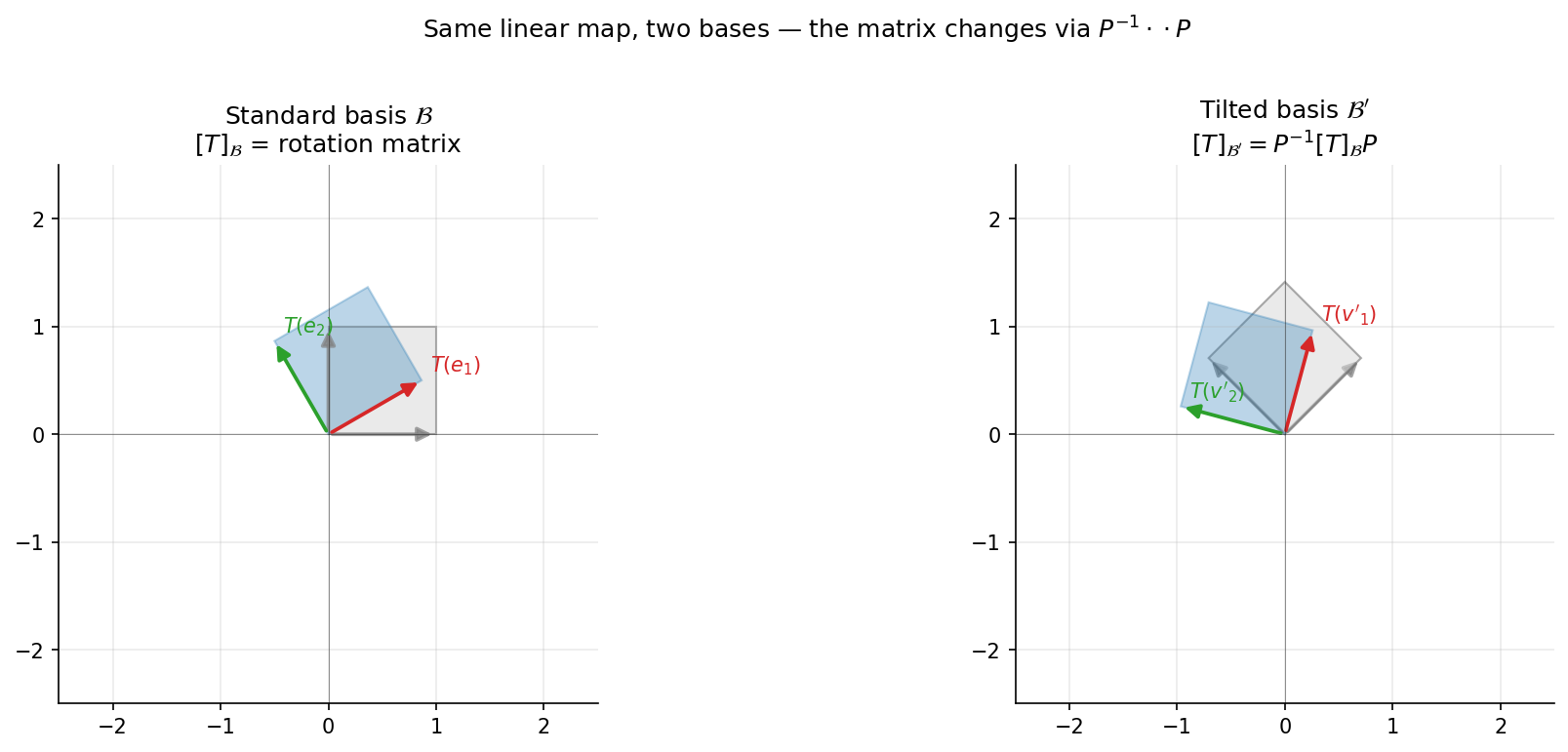
The formula is sometimes written , where and are the matrices in the two bases. This is the operation that says “translate input, apply, translate output back.” Two matrices related this way are called similar, and similarity is the matrix-side reflection of “same linear map, different basis.”
📝 Example 14 (Rotation in a Tilted Basis)
Let be rotation by in . Its matrix in the standard basis is
Now switch to the basis — the standard basis rotated by . The change-of-basis matrix from to the standard basis has the new basis vectors as columns:
This matrix is itself a rotation by , and a rotation is its own inverse-transpose: . The change-of-basis formula gives
Crucially, rotations commute with rotations: if you tilt the basis and apply a rotation, you get the same answer as if you apply the rotation and then tilt the basis. So , and the matrix is unchanged. This is the cleanest example of a similarity transformation that doesn’t change the matrix — and it reflects a structural fact about rotations: their action is the same in every orthonormal basis.
📝 Example 15 (Projection in a Non-Standard Basis)
Let be the orthogonal projection of onto the line . In the standard basis, , so
Now switch to the basis — the line and its perpendicular. In this basis the projection is trivial to describe: it sends the first basis vector to itself (it’s already on the line) and the second to zero (it’s perpendicular to the line). So
The same linear map has two very different matrices. The change-of-basis formula ties them together; a direct calculation (with the same as Example 14) verifies the relationship. This is also the cleanest possible example of a basis chosen to make a map simple — and it foreshadows the central question of the next topic: can we always find such a basis? The answer for diagonalizable maps is yes, and the basis vectors are the eigenvectors of the map. We will not develop that here, but Example 15 is the prototype that motivates the question.
💡 Remark 9 (Similar Matrices Are the Same Map)
Two matrices and are similar if there exists an invertible matrix with . By Theorem 8, similar matrices are exactly the matrices of the same linear map in different bases. Two consequences:
- Quantities that depend only on the underlying map are equal for similar matrices. These include the trace, the determinant, the rank, the nullity, the characteristic polynomial, and the set of eigenvalues. We list them here even though some haven’t been formally defined; the point is that they are invariants of the map, not of the bookkeeping.
- Quantities that depend on the choice of basis differ. These include the individual entries, the column space (as a specific subspace of , not its dimension), and the specific eigenvector representatives.
When you ask “what is true about the linear map,” you are asking about invariants of similarity. When you ask “what does this particular matrix look like,” you are asking about something basis-dependent that may not match what you’d see in a different basis. Distinguishing the two questions is most of the conceptual work of an applied linear-algebra course.
ML aside. Data whitening — multiplying centered data by , where is the sample covariance matrix — is a change of basis. In the original coordinates, the data has whatever covariance structure happens to be present; in the whitened coordinates, the covariance is the identity, meaning every direction has unit variance and every pair of directions is uncorrelated. Many algorithms behave better in the whitened basis — gradient descent on isotropic data has condition number , k-means clusters become equidistant in the natural sense, the Mahalanobis distance becomes the ordinary Euclidean distance. Choosing to whiten is choosing a basis in which the algebra is simpler. The same theorem (Theorem 8) describes how the data’s statistical properties transform under that change of basis — they don’t change in any deep sense, only their representation does.
10. Inner Products and Orthogonality
Everything in this topic so far has been algebraic — about addition, scalar multiplication, linear combinations, and the maps that respect those operations. None of it has involved measurement. We have not said how long a vector is, what angle two vectors make, or what it means for two vectors to be perpendicular. Those concepts require an additional structure on a vector space called an inner product, and adding that structure is what turns a vector space into something we can do geometry with: lengths, angles, projections, distances, and orthogonality.
The standard inner product on — the dot product — is the example we already know. Generalizing the dot product to a list of axioms reveals what makes it tick: it is symmetric (treats both inputs the same), linear in each argument, and positive-definite (a vector’s inner product with itself is non-negative, and zero only for the zero vector). Anything that satisfies those properties earns the name inner product, and the resulting theory works in exactly the same way as for the dot product. Three central theorems will come out of this: the Cauchy-Schwarz inequality (which makes “angle” well-defined), the orthogonal decomposition theorem (which makes orthogonal projection canonical), and the Gram-Schmidt process (which constructs orthonormal bases on demand).
📐 Definition 17 (Inner Product)
An inner product on a real vector space is a function satisfying:
- (Symmetry) for all .
- (Linearity in the first slot) for all and . By symmetry, the same holds in the second slot.
- (Positive-definiteness) for all , with equality if and only if .
A vector space equipped with an inner product is called an inner product space.
📐 Definition 18 (Induced Norm)
In any inner product space , the norm (or length) induced by the inner product is
Positive-definiteness (axiom I3) ensures that the square root is well-defined and that iff . A vector with is called a unit vector.
📝 Example 16 (Standard Inner Product on ℝⁿ)
The function — the familiar dot product — is an inner product on . Symmetry and bilinearity follow from the arithmetic of real numbers; positive-definiteness follows because , with equality only when every . The induced norm is the Euclidean norm , the length of the arrow from the origin to .
📝 Example 17 (L² Inner Product on C[a, b])
On the space of continuous functions , define
Symmetry and bilinearity follow from the linearity of integration. Positive-definiteness uses the fact that a non-negative continuous function with zero integral over must be identically zero — a fact established in Riemann Integral & FTC. The induced norm is , sometimes called the norm. Two functions are “orthogonal” in this inner product when — the orthogonality condition behind Fourier series (Fourier Series & Orthogonal Expansions).
The dot product satisfies , which the reader may know from Euclidean geometry as “the cosine of an angle is between and .” The same inequality holds for every inner product, with the same proof, and it is the inequality that lets us define the angle between two vectors in an arbitrary inner product space.
🔷 Theorem 9 (Cauchy-Schwarz Inequality)
For any vectors in an inner product space ,
with equality if and only if and are linearly dependent (one is a scalar multiple of the other, possibly zero).
Proof.
If , both sides are zero and equality holds trivially with and trivially dependent. Assume .
Consider the real-valued function
Expanding via bilinearity and symmetry,
This is a quadratic in that is always by positive-definiteness, so its discriminant is :
Simplifying gives , i.e.,
Taking square roots of non-negative numbers gives , which is the claimed inequality.
Equality holds iff the discriminant is exactly zero, iff the quadratic has a (double) real root, iff there exists with , iff (by positive-definiteness), iff and are linearly dependent.
The Cauchy-Schwarz inequality guarantees that the ratio lies in whenever both vectors are nonzero. So the formula
defines a well-defined angle between any two nonzero vectors in any inner product space. This is the angle that the dot product “measures” in — but the formula and the result extend to function spaces, sequence spaces, and any other inner product space. The angle is part of the structure, not a Euclidean artifact.
The special case where the angle is — equivalently, the inner product is zero — earns the name orthogonality and is the most-used geometric concept in linear algebra.
📐 Definition 19 (Orthogonality and Orthogonal Complement)
Two vectors in an inner product space are orthogonal, written , if .
A set is orthogonal if every pair is orthogonal; orthonormal if it is orthogonal and every has unit norm. An orthonormal basis is a basis that is orthonormal.
For a subspace , the orthogonal complement is
is itself a subspace of (verify: closure under addition and scalar multiplication follow from bilinearity of the inner product).
The geometric content of orthogonality is “perpendicular.” Two orthogonal nonzero vectors point in directions that share no component — projecting one onto the other gives zero. The orthogonal complement of a subspace is the set of vectors perpendicular to every vector in ; in , the orthogonal complement of a line is a plane and of a plane is a line. The remarkable fact, which the next theorem packages, is that splits cleanly into and .
🔷 Theorem 10 (Orthogonal Decomposition)
Let be a finite-dimensional inner product space and a subspace. Then every has a unique decomposition
The map is the orthogonal projection of onto , and it is a linear map. Symbolically, (direct sum decomposition).
We will use Theorem 10 below in the proof of Gram-Schmidt; the proof of Theorem 10 itself is a constructive argument using the Gram-Schmidt process (an example of theorems that are best proved by their algorithm), so we postpone the formal proof to a follow-up topic (Hilbert Spaces) where the infinite-dimensional version becomes the main event. In finite dimensions, the proof reduces to constructing an orthonormal basis of , extending it to one of , and reading off the decomposition.
The construction of an orthonormal basis from any old basis is the Gram-Schmidt process — an algorithm so important that it earns its own theorem.
🔷 Theorem 11 (Gram-Schmidt Produces an Orthonormal Basis)
Let be a basis of an inner product space . Define vectors and recursively:
and for :
Then is an orthonormal basis of , and for every , .
Proof.
We prove by induction on that (a) is orthonormal, and (b) .
Base case (). Since is a basis, , so and is well-defined. By construction, , so the singleton is orthonormal. The span condition is immediate: , since is a nonzero scalar multiple of .
Inductive step. Assume the claim holds for indices ; that is, is orthonormal with . Examine the construction:
Orthogonality of to each for . Take the inner product of with :
By the inductive orthonormality of , (one when , zero otherwise). The sum collapses to a single nonzero term at :
So is orthogonal to each for .
Non-vanishing of . Suppose for contradiction . Then , so . But is a basis, so its elements are linearly independent, and cannot lie in the span of the earlier . Contradiction. So and , making well-defined and a unit vector.
Orthonormality of the full set. The orthogonality of to each for carries to by scaling (the inner product is bilinear). Combined with and the inductive orthonormality, is orthonormal.
Span condition. By construction, is a linear combination of and (which, by induction, span ). So . Conversely, is recoverable from and the earlier (rearrange the Gram-Schmidt formula), so . Together with the inductive span condition for the first vectors, this gives .
By induction, the claim holds for all up to . At , is an orthonormal basis of , completing the proof.
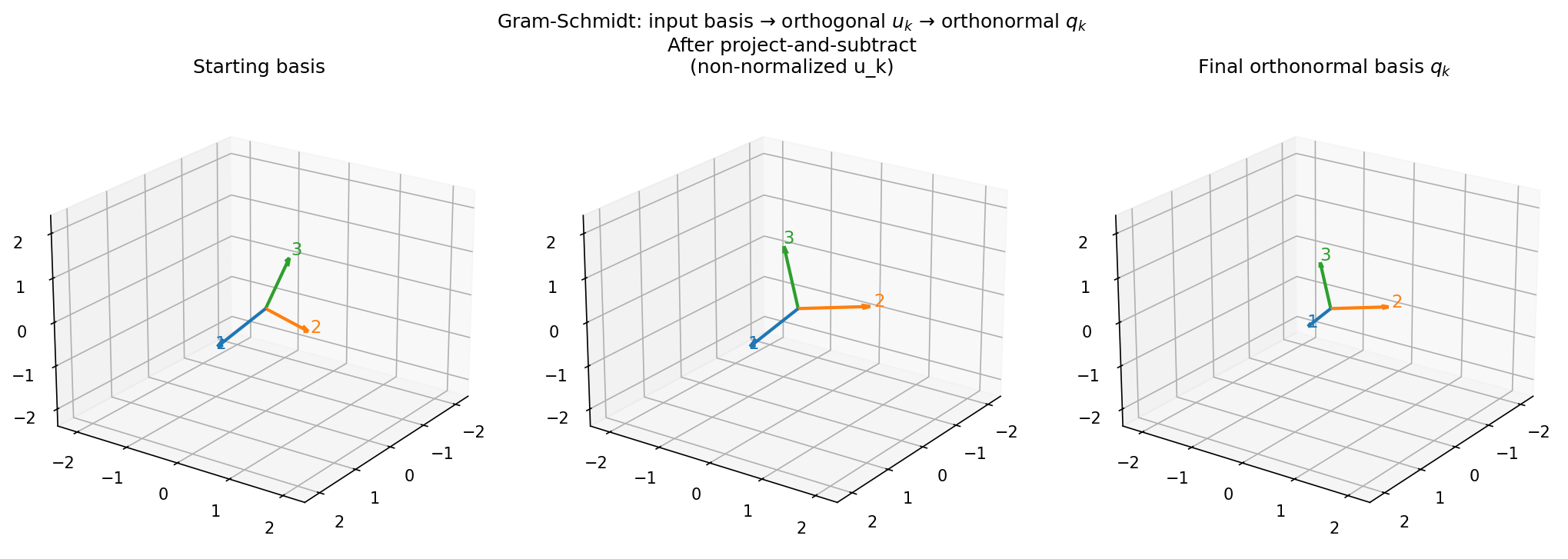
The Gram-Schmidt process is the canonical way to manufacture an orthonormal basis on demand. The viz below steps through the process on a skewed input basis of , with each rendered in grey, the projections being subtracted in orange, the intermediate in blue, and the finalized in green. The accumulating orthonormal basis is reported in a side panel as the algorithm runs.
The Gram-Schmidt running example from notebook §8 — independent and visibly skewed.
Three input basis vectors of ℝ³ shown in grey. Click "Next step" to begin Gram-Schmidt — or "Run to end" to animate the whole process.
- (none yet)
💡 Remark 10 (QR Factorization)
If we apply Gram-Schmidt to the columns of an matrix (with and full column rank), the orthonormal vectors become the columns of an matrix with orthonormal columns. The relationship between and takes the form
where is an upper-triangular matrix whose entries are exactly the coefficients that Gram-Schmidt computes: for and for . This is the QR factorization of — the orthogonal-triangular decomposition that powers numerical least-squares solvers, eigenvalue iterations, and many other algorithms. We will not develop QR in detail here; the Numerical Linear Algebra literature (Trefethen & Bau) treats it in full, and the spectral theorems of the next track topic depend on it implicitly.
ML aside. Cosine similarity — the dominant similarity metric for embedding spaces in modern ML (Word2Vec, sentence-transformers, retrieval-augmented generation, recommender systems) — is the cosine of the angle between two vectors, exactly the formula derived from Cauchy-Schwarz above:
The Cauchy-Schwarz inequality is what guarantees this quantity lies in — and is what makes the metric well-defined regardless of vector dimension. Two further uses: the triangle inequality (a corollary of Cauchy-Schwarz, derivable by expanding the squared norm) controls how embeddings compose under addition, which is the constraint behind compositional embeddings like Word2Vec’s analogy property “king − man + woman ≈ queen.” And the orthogonality of residual to design-matrix columns in least-squares regression — equivalent to the orthogonal-decomposition theorem applied to projected onto — is the geometric statement behind the normal equations, which the next section will unpack.
Where this leads. We have built a lot of geometric machinery — angles, lengths, orthogonality, orthogonal projections, orthonormal bases. The most natural next question is: given a linear map , are there directions in the space that does not rotate? Directions where for some scalar — the map merely stretches the vector by a factor of but does not reorient it. Such a direction is a 1-dimensional invariant subspace, and the vectors along it are called eigenvectors of with eigenvalue . For some maps (e.g. projections, rotations by or , scalings) such directions abound; for others (rotation by in ) no real direction is fixed. The systematic theory of when eigenvectors exist, how many there are, and what they tell us about a map is the content of the next topic, Eigenvalues & Eigenvectors. The spectral theorem for symmetric matrices — the headline result of that topic — says that a symmetric matrix has an orthonormal basis of eigenvectors, tying together the orthogonality of this section with the eigenvalue picture of the next.
11. Connections to Machine Learning
Linear algebra is the most heavily invoked piece of mathematics in machine learning. The inline ML asides at the end of each section have signposted specific connections one at a time — neural-network layers as linear maps, projections as bias-free regression, deep linear networks as products of matrices, normalizing flows as Jacobian-volume preservation, autoencoders as rank constraints, embeddings as choices of basis, cosine similarity as the Cauchy-Schwarz quotient. This section consolidates three of the largest connections into stand-alone treatments that draw on the full apparatus of §§1-10.
11.1 Least Squares as Orthogonal Projection
The single most common use of linear algebra in applied work is ordinary least squares regression. Given data with design matrix and response vector , OLS solves the minimization
The algebraic answer is the closed-form expression — derivable by setting the gradient to zero and inverting. That algebraic derivation is correct, but it conceals the reason the formula looks the way it does. The reason is geometric: is the unique vector of coefficients that puts at the orthogonal projection of onto the column space of — and the formula above is just the algebraic shadow of that projection.
Here is the geometric story written out. Let denote the column space of (a subspace of of dimension ). Every reachable prediction lives in — that is the definition of the column space. The squared error is the squared distance from to the candidate prediction. By the orthogonal-decomposition theorem (Theorem 10), , so has a unique decomposition with and . The minimum-distance point in to is exactly — the orthogonal projection — with distance .
So the OLS prediction is , and the residual is orthogonal to every column of . Writing the orthogonality condition columnwise gives the normal equations:
When has full column rank, is invertible (by Corollary 1 applied to the matrix , whose columns are independent iff ‘s columns are) and we recover . The algebraic formula is the geometry rewritten in coordinates.
📝 Example 18 (A Solved Least-Squares Problem)
Fit a line to the four data points . Set up the design matrix and response,
Compute the normal-equation ingredients:
Invert the matrix: , so
Apply to :
So and , fitting the line . The notebook (cell §9) plots the four points, the line, and the four residual arrows orthogonal to , making the orthogonality of the residual visible.
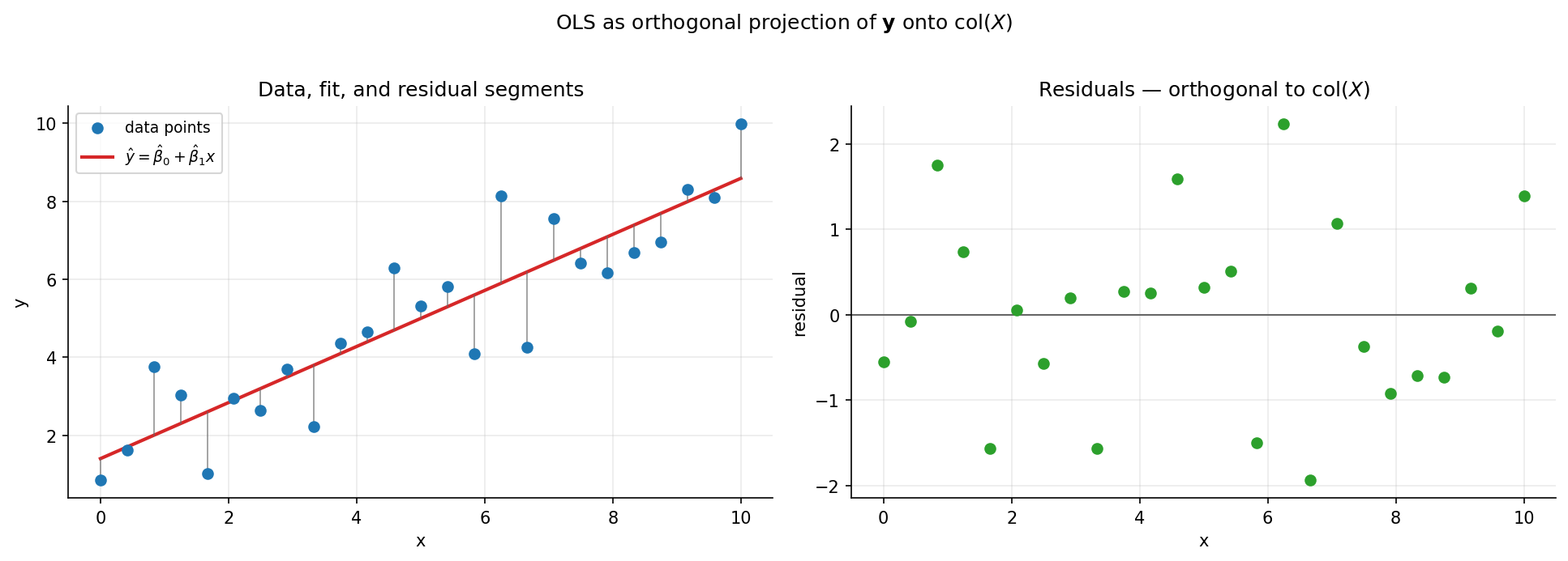
The geometric story extends in three useful directions. The orthogonal projection is itself a linear map; its matrix in the standard basis is the projection matrix , and the hat matrix has trace equal to — the “effective number of parameters” in classical statistics. The residual matrix is also a projection (onto ). And when is rank-deficient, the formula fails — exactly the diagnosis from Example 13 (underdetermined regression), and exactly the situation where ridge or lasso regularization steps in. Every applied-statistics technique stacked on top of linear regression — diagnostics, leverage, influence, generalized inverses — descends from this orthogonal-projection geometry. regression-fundamentals →
11.2 Embeddings as Choices of Basis
A modern ML embedding maps discrete objects (words, sentences, users, items, documents) to vectors in , where is typically a few hundred to a few thousand. Word2Vec uses ; BERT’s [CLS] token lives in ; the OpenAI text-embedding APIs return -dimensional vectors. From the linear-algebra perspective, an embedding is a choice of basis for the latent space — the axes of are implicit basis vectors, chosen by training to make geometrically nearby vectors semantically similar.
This framing has immediate consequences. The famous Word2Vec analogy property, , is a linear-combination statement in : it says that the vector difference is approximately equal to , both representing the abstract “royalty” direction in the latent basis. The triangle inequality from §10 (Cauchy-Schwarz corollary) constrains how exactly this can hold — perfect equality would require the four words to lie on a parallelogram, which they don’t. The approximation works because the trained basis has learned to align such relationships with linear-combination operations.
The same picture explains why PCA (principal component analysis) is useful as embedding post-processing. PCA finds an orthonormal basis (the principal components) ordered by variance, and the first few components capture the directions in which the embedding distribution is most spread out. Re-expressing the embedding in this principal basis is a change of basis (§9) — the same data lives in a new coordinate system. We are not yet in a position to compute the principal components; they are eigenvectors of the covariance matrix, which belongs to the next topic. But the setup — pick a basis adapted to the data’s structure — is exactly the change-of-basis idea developed here. embeddings →
11.3 Quadratic Local Approximation of Loss
Near a critical point of a smooth loss function , Taylor expansion gives the second-order approximation
where is the Hessian matrix at the critical point (the gradient term vanishes because is critical). The quadratic form controlling the shape of the loss surface near is — when is positive-definite — exactly the squared norm induced by the inner product . So the local geometry of optimization is the inner-product geometry from §10, with playing the role of the inner product.
Three consequences worth noting. First, the level sets of the quadratic approximation are ellipsoids whose principal axes are the eigenvectors of — exactly the basis from §9 in which becomes diagonal. Gradient descent’s convergence rate is controlled by the condition number of (the ratio of largest to smallest eigenvalue), and this condition number is the same number that quantifies “how badly tilted the ellipsoid is” — a basis-invariant quantity, but one whose computation requires diagonalization. Second, Newton’s method uses the inverse Hessian to rescale gradient steps into the basis where the loss is locally isotropic: takes one step to a quadratic local minimum, by construction. Third, adaptive optimizers like Adam and RMSProp can be read as approximate Hessian rescalings — they whiten the gradient using running statistics that mimic , exactly the change of basis from the data-whitening ML aside in §9.
The whole story is: a quadratic form is an inner product is the geometry of optimization near a critical point. Once you know that, every line in an optimization textbook becomes a statement about basis-adapted geometry. gradient-descent → neural-network-basics →
12. Connections to Statistics
The single most important statistical object derived from linear algebra is the sample covariance matrix. Given mean-centered data (rows are observations, columns are features, and each column has mean zero), the sample covariance is
This is a Gram matrix — specifically, the matrix of pairwise inner products of the columns of , scaled by . As a Gram matrix, inherits the full structure developed in §10: it is symmetric, positive-semi-definite, and rank-equal to . Its column space is the subspace of that the centered data actually inhabits, and its rank measures how many independent feature directions are present in the data — a rank-nullity statement applied to a covariance estimate. When is full-rank (positive-definite), it defines an inner product on ; the induced norm is the Mahalanobis distance, which weights coordinates by their inverse variance and is the right notion of distance when feature scales differ. covariance-correlation →
The method of moments and the broader theory of M-estimation (maximum likelihood, generalized method of moments) rely on the matrix machinery developed here in a different way. The asymptotic variance of an M-estimator has the sandwich form , where is a Jacobian-like matrix and is a covariance of score functions. The inverse requires to be invertible — which by Corollary 1 is the identifiability condition for the estimator. The quadratic form is the asymptotic variance of any linear contrast of the parameters, and again the inner-product geometry from §10 determines confidence-region geometry. method-of-moments →
Finally, linear regression inference — the F-tests, t-tests, and confidence intervals attached to the OLS estimator — reads off directly from the rank of and the inner-product structure of the residual space. The residual sum of squares lives in , whose dimension is ; this is the famous "" degrees of freedom appearing in the denominator of the unbiased variance estimator. Every classical-statistics formula in linear regression — leverage, influence, the F-distribution of the test statistic, the geometry of nested-model comparison — descends from the orthogonal-decomposition theorem applied to the column space and its complement. linear-regression-inference →
13. Where This Leads
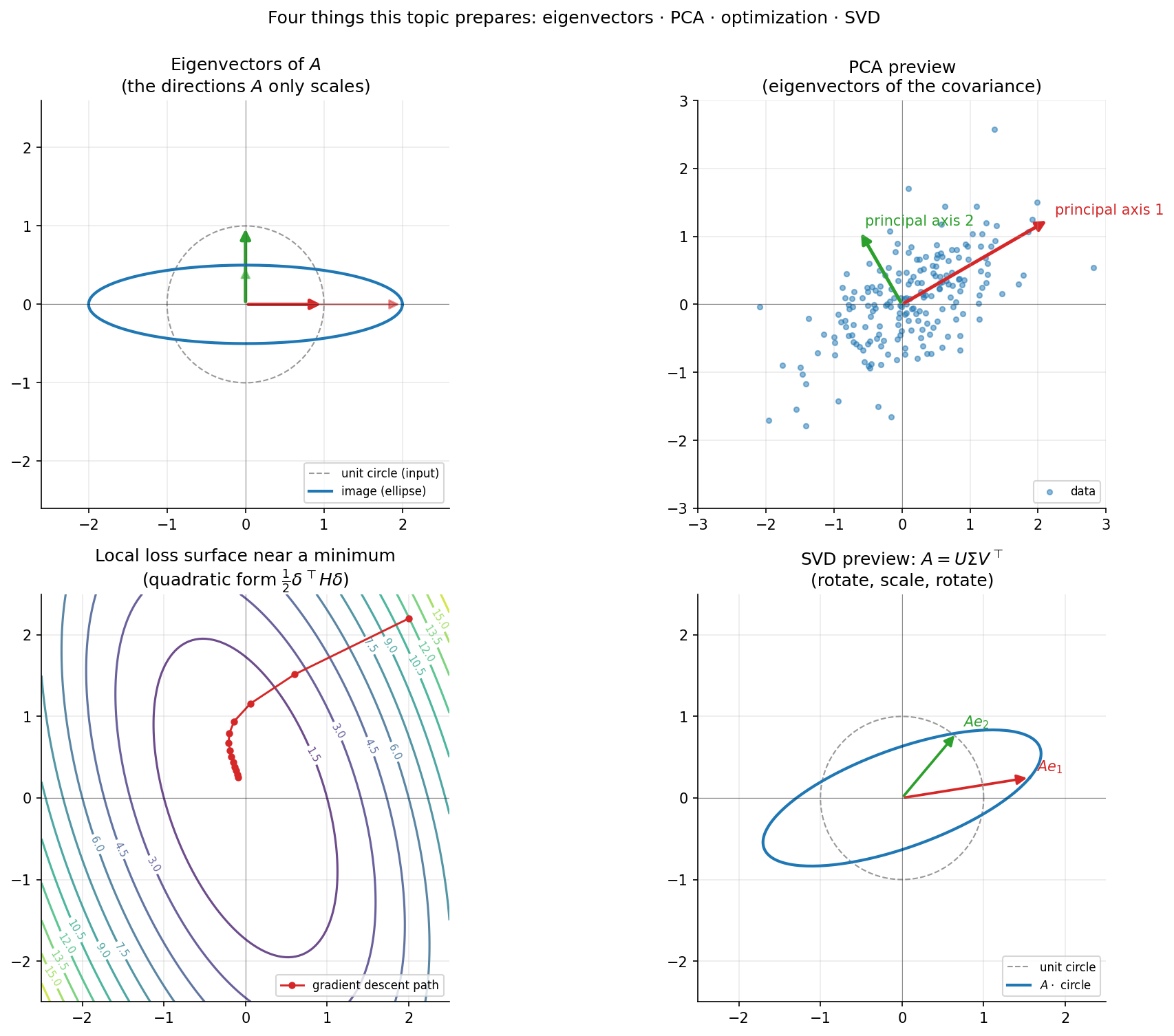
This topic built the foundation. Three downstream directions extend the apparatus, each with its own topic on this site or its sister sites.
Eigenvalues and Eigenvectors is the immediate next topic on this track. The animating question is: given a linear map , can we find a basis of in which has a particularly simple matrix? For some maps the answer is yes, and the basis is a basis of eigenvectors — directions that merely scales, , without rotation. In that basis the matrix is diagonal, with the diagonal entries being the eigenvalues. The full theory — characteristic polynomials, multiplicities, diagonalizability criteria, the spectral theorem for symmetric matrices, defective maps and Jordan canonical form — is the content of the next topic. Two of this topic’s loose ends close immediately there: Example 15’s projection-becomes-diagonal observation is the prototype of the spectral theorem, and the eigenvalue framing for the Hessian condition number (§11.3) becomes concrete.
Singular Value Decomposition (SVD) generalizes the eigenvalue picture to rectangular matrices. Every real matrix factors as , where is orthogonal, is orthogonal, and is diagonal with non-negative entries called the singular values. The SVD says that every linear map between inner-product spaces factors as “rotate, scale along orthogonal axes, rotate again” — a remarkable structural theorem that underpins low-rank approximation, principal component analysis, recommendation systems, latent-semantic indexing, and many more. We do not develop SVD here; it is the natural sequel to Eigenvalues and is best treated as a separate topic.
Quadratic forms reappear in optimization through the Hessian and the second-derivative test, in geometry through curvature (the Gaussian curvature of a surface is the determinant of a quadratic form), and in statistics through the multivariate Gaussian distribution (whose density is , a quadratic form in disguise). The apparatus built in this topic — inner products, symmetric matrices, the geometry of orthonormal bases — is the entry pass to every quadratic-form result downstream.
Beyond this topic, functional analysis (Track 8) lifts every finite-dimensional construction here into infinite dimensions. Inner products become bounded sesquilinear forms; orthonormal bases become Hilbert-space bases; the orthogonal-decomposition theorem becomes the projection theorem for closed subspaces; the rank-nullity theorem becomes the open-mapping theorem and the index theorem. The transition from finite to infinite dimensions is non-trivial — questions of convergence and completeness arise that have no finite-dimensional analog — but the language developed here is exactly the language that infinite-dimensional theory inherits. Metric Spaces, Normed & Banach Spaces, Inner Product & Hilbert Spaces, and Calculus of Variations carry the story forward.
The finite-dimensional theory is complete in its own right — every theorem in this topic stands on its own and has unconditional applications, from solving linear systems to fitting regression models. But the apparatus also serves as the warm-up for a deeper story whose chapters are written elsewhere on this site. Eigenvalues & Eigenvectors is next.
Connections & Further Reading
Where this leads — next in formalCalculus
On to formalStatistics — where this calculus powers inference
Method Of Moments
Sandwich variance formulas of the form A⁻¹BA⁻¹ᵀ in M-estimation depend on the matrix inverse properties, quadratic-form positivity, and rank conditions developed here. The inner-product framework supplies the geometry; rank-nullity supplies identifiability.
Covariance Correlation
The covariance matrix Σ of a mean-centered random vector is the Gram matrix XᵀX/n of the centered data. Its rank equals the dimension of the linear span of the observations, and its column space is the subspace the data actually inhabits — both rank-nullity statements.
Linear Regression Inference
The OLS estimator β̂ = (XᵀX)⁻¹Xᵀy is the orthogonal projection of y onto the column space of the design matrix X. Its sampling distribution, the geometry of residuals, and the F-test all read off the inner-product structure and the rank of X established in this topic.
On to formalML — where this calculus powers ML
Neural Network Basics
A feedforward layer x ↦ σ(Wx + b) is the composition of a linear map W with a componentwise nonlinearity. The column space of W is what the layer can output linearly; the rank of W is the number of independent features that survive. Reading layers geometrically is reading matrices as linear maps.
Gradient Descent
Gradient descent θ ← θ − η∇L lives in a finite-dimensional inner-product space. Convergence rates depend on quadratic-form approximations of the loss, which are inner products in disguise; the condition number κ controlling speed is a quadratic-form quantity, not an algebraic one.
Regression Fundamentals
Ordinary least squares is the orthogonal projection of y onto col(X). The closed-form β̂ = (XᵀX)⁻¹Xᵀy is the algebraic shadow of the geometric statement P_col(X) y = Xβ̂, and the residual y − Xβ̂ is orthogonal to every column of X — exactly the orthogonal complement decomposition.
Embeddings
Word2Vec, BERT, and graph-embedding methods produce vectors in ℝᵈ where cosine similarity ⟨u, v⟩ / (‖u‖ ‖v‖) measures semantic proximity. Choosing an embedding is choosing a basis for the latent space; analogies (king − man + woman ≈ queen) are linear-combination statements; PCA and SVD post-processing are spectral operations on the embedding matrix.
References
- book Axler, S. (2024). Linear Algebra Done Right The canonical determinant-free linear-algebra textbook. Chapters 1–6 cover everything in this topic with the geometric, coordinate-free perspective we use here. The eigenvalue-first reordering is influential but not directly followed.
- book Strang, G. (2023). Introduction to Linear Algebra Strang's column-space-first treatment is the closest published match to our pedagogical line. Chapter 3 (rank, nullspace) and Chapter 4 (orthogonality, projection) are the direct sources for our rank-nullity and least-squares exposition.
- book Halmos, P. R. (1958). Finite-Dimensional Vector Spaces The classical reference for the abstract treatment of finite-dimensional vector spaces. Read for the axiomatic discipline; not for pedagogy.
- book Hoffman, K. & Kunze, R. (1971). Linear Algebra Mathematically heaviest of the standard references — full proofs, no shortcuts. Useful for cross-checking rank-nullity and change-of-basis statements.
- book Lang, S. (1987). Linear Algebra Lang's treatment is compact and abstract. Chapters on bilinear forms and inner products are the sources for our framing of inner products as a structure on a vector space rather than a derived concept.
- book Meyer, C. D. (2000). Matrix Analysis and Applied Linear Algebra The computational and applied reference. Chapter 5 on orthogonality is the source for the Gram-Schmidt presentation, and the determinant-as-volume framing in §4 is taken almost directly from here.
- book Trefethen, L. N. & Bau, D. (1997). Numerical Linear Algebra Trefethen's columns-as-vectors viewpoint is the cleanest available exposition of matrix-as-linear-map. We borrow the visual framing of matrix multiplication as repeated linear combinations of columns.